Comprehensive Guide to Polynomial and Rational Functions
Unit 1: Polynomial and Rational Functions
Change in Tandem & Rates of Change
Functions and Variation
Function: A mathematical relationship mapping a set of inputs (Domain, independent variable $x$) to a set of outputs (Range, dependent variable $y$) such that every input maps to exactly one output.
In AP Precalculus, we analyze how input and output values change in tandem (together). We look at the direction of change and the rate at which that change occurs.
- Increasing: As inputs increase ($x o →$), outputs increase ($y o ↑$). Technically: $f(b) > f(a)$ whenever $b > a$.
- Decreasing: As inputs increase ($x o →$), outputs decrease ($y o ↓$). Technically: $f(b) < f(a)$ whenever $b > a$.
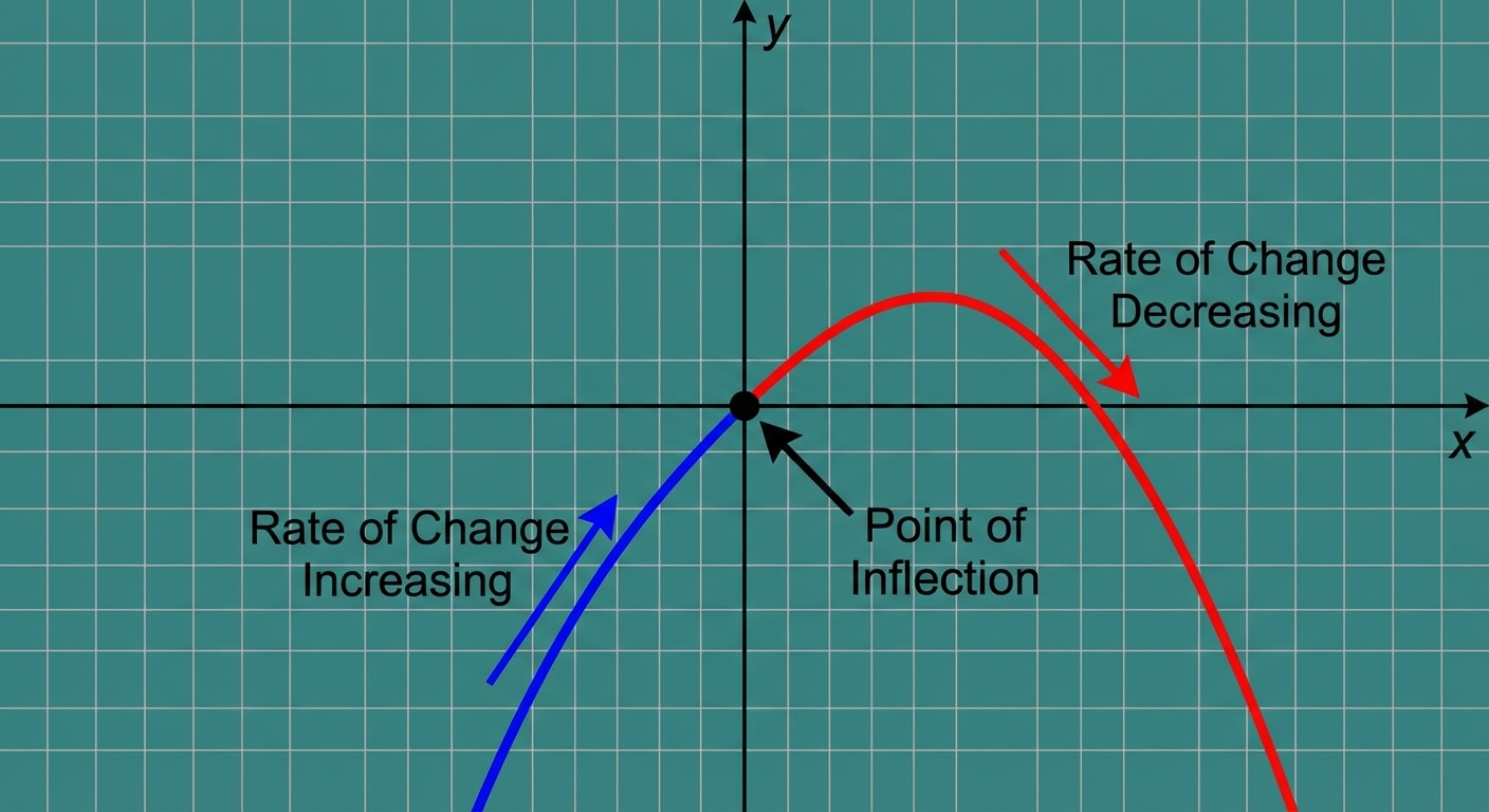
Concavity and Rate of Change
The "shape" or curvature of a function is determined by how its rate of change behaves.
- Concave Up: The rate of change is increasing. The graph bends upward (like a cup).
- Slope gets more positive (or less negative).
- Concave Down: The rate of change is decreasing. The graph bends downward (like a frown).
- Slope gets less positive (or more negative).
Average Rate of Change (AROC)
The AROC represents the slope of the secant line connecting two points on a graph.
| Function Type | Rate of Change Behavior |
|---|---|
| Linear | Constant rate of change (AROC is the same for any interval). |
| Quadratic | Linear rate of change (The AROC changes at a constant rate). |
| Cubic/Higher | The rate of change itself changes at a changing rate. |
Common Mistakes
- Confusing Concavity with Direction: A function can be decreasing but concave up (e.g., the left side of $y=x^2$).
- AROC intervals: Remember that AROC is strictly calculated over a closed interval $[a, b]$. It is not the instantaneous slope at a single point (which is a derivative).
Polynomial Functions
Definitions and Degree
A polynomial function is in the form $p(x) = an x^n + a{n-1} x^{n-1} + \dots + a_0$, where $n$ is a non-negative integer and coefficients are real numbers.
- Degree ($n$): The highest exponent. Determines the maximum number of zeros and the general shape.
- Leading Coefficient ($a_n$): The coefficient of the term with the highest degree.
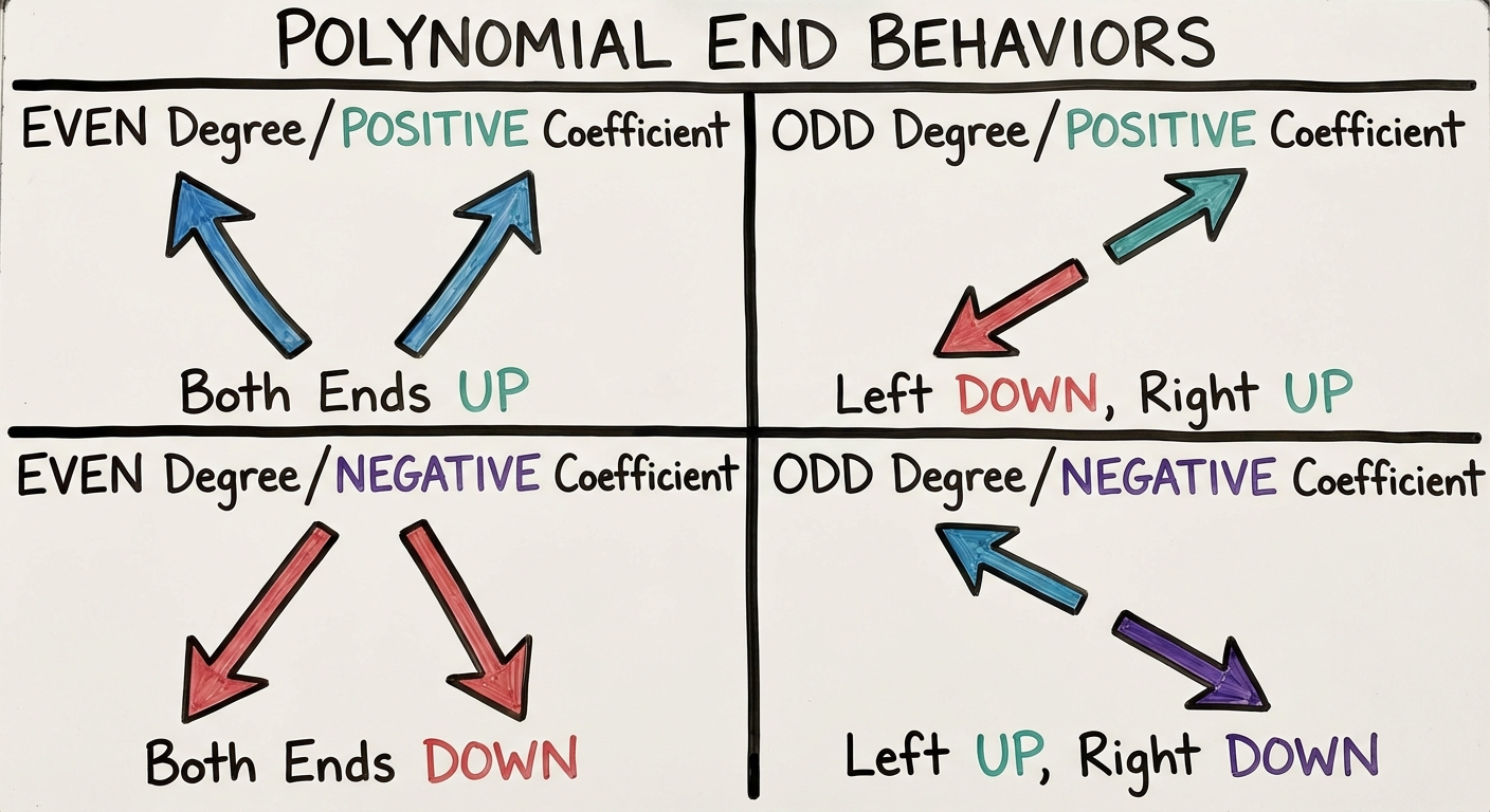
End Behavior (The Leading Term Test)
The long-run behavior of a polynomial (as $x o \pm\infty$) is determined solely by the leading term.
We express end behavior using limit notation:
Case 1: Even Degree ($n$ is even)
- Positive $an$: $\lim{x \to \infty} f(x) = \infty$ and $\lim_{x \to -\infty} f(x) = \infty$ (Up/Up)
- Negative $an$: $\lim{x \to \infty} f(x) = -\infty$ and $\lim_{x \to -\infty} f(x) = -\infty$ (Down/Down)
Case 2: Odd Degree ($n$ is odd)
- Positive $an$: $\lim{x \to \infty} f(x) = \infty$ and $\lim_{x \to -\infty} f(x) = -\infty$ (Down/Up)
- Negative $an$: $\lim{x \to \infty} f(x) = -\infty$ and $\lim_{x \to -\infty} f(x) = \infty$ (Up/Down)
Zeros and Multiplicity
Fundamental Theorem of Algebra: A polynomial of degree $n$ has exactly $n$ complex zeros (counting multiplicity).
If $p(a) = 0$, then $x = a$ is a root, and $(x - a)$ is a factor.
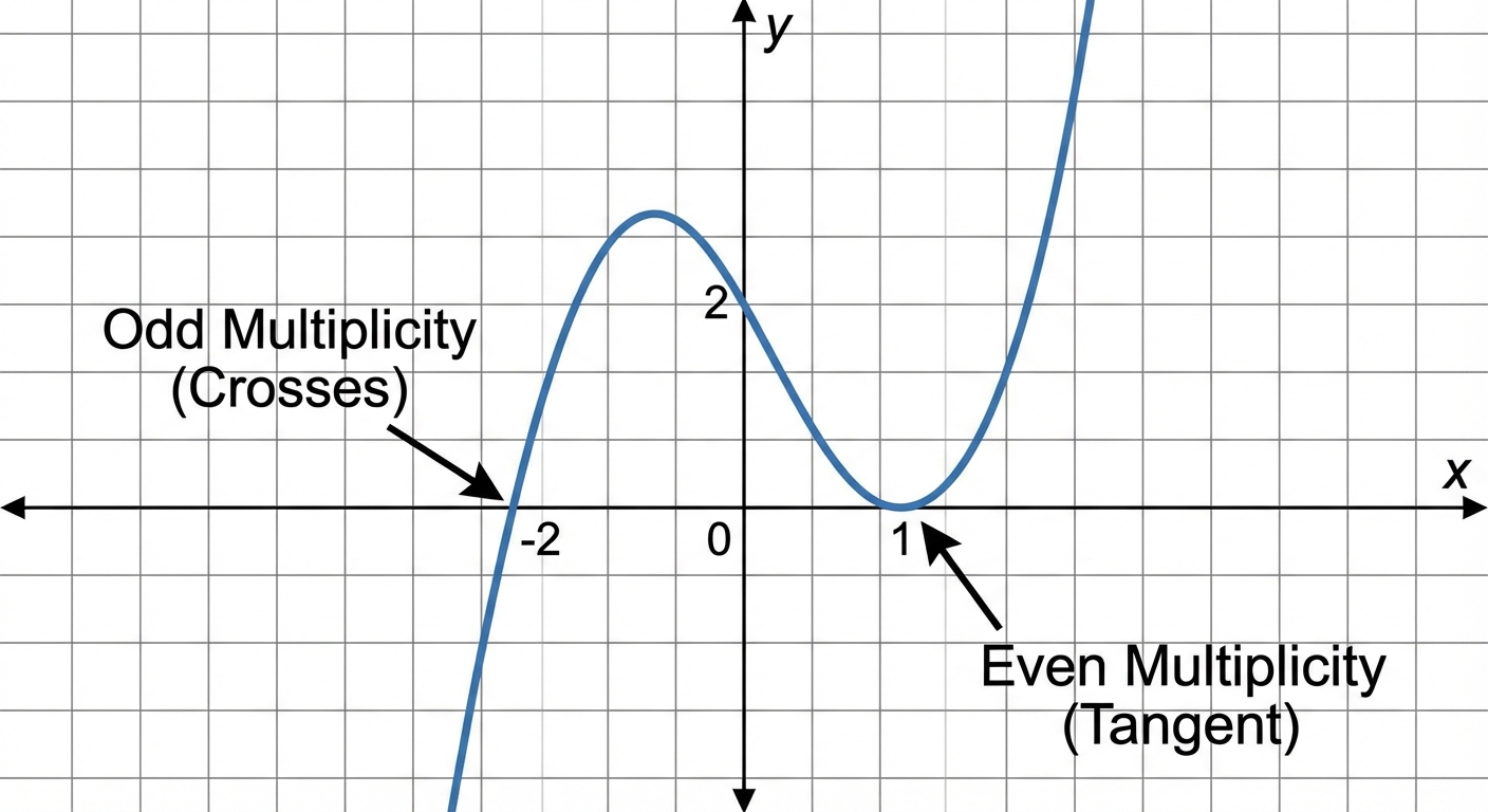
Multiplicity behavior on the graph:
- Odd Multiplicity (e.g., $(x-3)^1, (x-3)^3$): The graph crosses the x-axis at the root.
- Even Multiplicity (e.g., $(x-3)^2, (x-3)^4$): The graph is tangent to (or bounces off) the x-axis at the root.
Extrema and Inflection Points
- Local Extrema (Max/Min): Turning points where the function changes from increasing to decreasing (max) or vice versa (min). A polynomial of degree $n$ has at most $n-1$ turning points.
- Point of Inflection: Use this term carefully. This is where the concavity changes. A polynomial of degree $n$ usually has up to $n-2$ inflection points.
Rational Functions
Definition
A rational function is a ratio of two polynomials:
where $q(x) \neq 0$.
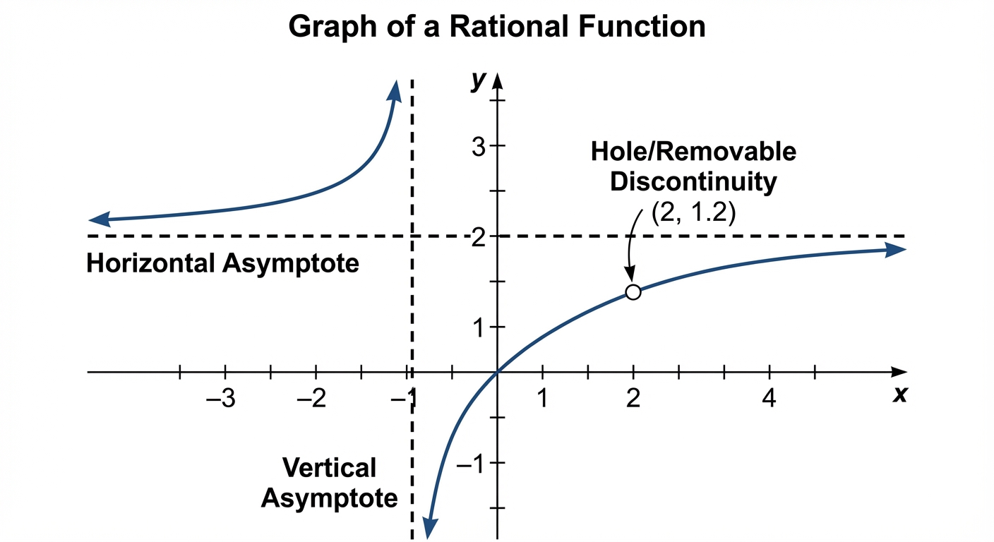
Discontinuities and Asymptotes
Identify features by analyzing the factors of the numerator and denominator.
1. Vertical Asymptotes (VA):
Occur at x-values where the denominator is zero, but the numerator is not zero. The graph shoots to $\infty$ or $-\infty$.
- Notation: $\lim_{x \to a^-} f(x) = \pm \infty$
2. Holes (Removable Discontinuities):
Occur at x-values where both the numerator and denominator are zero (a common factor cancels out).
- To find the y-coordinate of the hole: Cancel the factor and evaluate the simplified function at that x-value.
3. X-Intercepts:
Occur where the numerator is zero, but the denominator is not zero.
End Behavior (Horizontal and Slant Asymptotes)
Compare the degree of the numerator ($n$) and the degree of the denominator ($m$).
| Condition | Asymptote | Behavior |
|---|---|---|
| $n < m$ | Horizontal Asymptote at $y = 0$ | The x-axis is the asymptote. |
| $n = m$ | Horizontal Asymptote at $y = \frac{an}{bm}$ | Ratio of leading coefficients. |
| $n > m$ | Slant (Oblique) Asymptote | Found by polynomial long division (quotient is the line). |
Common Mistakes
- Hole vs. VA: Failing to cancel common factors first. If $(x-2)$ is in top and bottom, it's usually a hole, not a vertical asymptote.
- Crossing Asymptotes: A graph can cross a horizontal asymptote (local behavior), but it will approach it in the long run (end behavior). A graph generally does not cross a vertical asymptote.
Equivalent Representations & Algebra
Polynomial Long Division
Used to rewrite rational functions to find slant asymptotes or end behavior models.
If the degree of the numerator is exactly one higher than the denominator, the quotient (ignoring the remainder) is the equation of the Slant Asymptote.
Binomial Theorem
Useful for expanding binomials like $(x+a)^n$ without repetitive multiplication. The coefficients follow Pascal's Triangle.
Example for $n=3$:
Transformations of Functions
We transform a parent function $f(x)$ using the structure:
- Vertical Shift ($k$): Up if $k > 0$, down if $k < 0$. Affects Range/y-intercepts.
- Horizontal Shift ($h$): Right if $(x-h)$, Left if $(x+h)$. Affects Domain/x-intercepts.
- Vertical Dilation ($a$):
- $|a| > 1$: Vertical Stretch.
- $|a| < 1$: Vertical Compression.
- $a < 0$: Reflection over the x-axis.
- Horizontal Dilation ($b$):
- $|b| > 1$: Horizontal Compression by factor $1/b$.
- $|b| < 1$: Horizontal Stretch by factor $1/b$.
- $b < 0$: Reflection over the y-axis.
Crucial Note on Order: Always factor out the $b$ value inside the function.
- Wrong: $f(2x - 4)$ looks like a shift right by 4.
- Right: $f(2(x - 2))$ reveals it is a shift right by 2 and horizontal compression by $1/2$.
Function Model Selection & Assumptions
When given a data set or word problem, choose the model based on the rate of change.
- Linear: Constant first differences. Constant rate of change.
- Quadratic: Constant second differences. Modeling areas, projectile motion, or symmetric data with a peak/valley.
- Polynomial (Cubic/Quartic): First/second differences generally linear/quadratic. Used for complex curves with multiple turning points or volume constraints.
- Rational: Inversely proportional relationships (e.g., $y = k/x$). As one variable increases, the other decreases towards a limit.
Assumptions and Domain Restrictions
Mathematical models often require domain restrictions to fit reality:
- Contextual: Time cannot be negative; Area cannot be negative.
- Mathematical: Denominators $\neq 0$; Even roots of negative numbers are imaginary.
- Rounding: When a model predicts continuous data (like 2.5 people), we must interpret the integer validity of the result.