AP Bio Unit 8: Population Dynamics and Growth Models
Fundamentals of Population Ecology
Populations are dynamic entities. In AP Biology, understanding Population Ecology requires mastering how populations interact with their environment and how they change over time. By definition, a population consists of a group of individuals of the same species living in the same general area, relying on the same resources, and heavily influenced by similar environmental factors.
Key Variables in Population Dynamics
To mathematically describe a population, we look at several specific factors. This is often summarized by the equation:
Where:
- $N$: Population Size
- $B$: Births
- $D$: Deaths
- $I$: Immigration (entering the population)
- $E$: Emigration (leaving the population)
In most AP Biology exam scenarios, we simplify this by assuming immigration and emigration cancel each other out, focusing primarily on birth and death rates.
Population Growth Models
The College Board emphasizes the quantitative ability to calculate and graph population growth. You must differentiate between two specific models: Exponential and Logistic growth.
1. Exponential Growth (The J-Curve)
Exponential growth describes a population growing in an idealized environment with unlimited resources. Here, individuals reproduce at their physiological maximum capacity.
- Shape: J-shaped curve.
- Conditions: No external limits (food, space, predation).
- Example: Bacteria in a fresh culture; an invasive species entering a new habitat with no predators.
The Formula:
- $dN/dt$: The rate of population change over time (slope of the line).
- $r_{max}$: The maximum per capita growth rate (intrinsic rate of increase).
- $N$: Current population size.
Note: As the population size ($N$) increases, the rate of growth ($dN/dt$) increases, even if the per capita rate ($r$) remains constant. This is why the graph gets steeper.
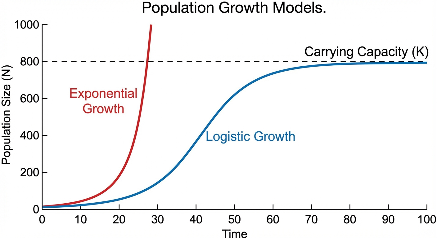
2. Logistic Growth (The S-Curve)
In the real world, resources are rarely unlimited. As a population grows, resources become scarce, and the growth rate creates a sigmoid (S-shaped) curve.
- Carrying Capacity ($K$): The maximum population size that a particular environment can sustain.
- Mechanism: As $N$ approaches $K$, the growth rate slows down. If $N = K$, the population growth rate is zero.
The Formula:
- The Modifier $\frac{K-N}{K}$: This term represents the "unused portion" of the carrying capacity.
- If $N$ is small (near 0), the term is close to 1, acting like exponential growth.
- If $N$ equals $K$, the term becomes 0, and growth stops.
Factors Affecting Population Density
A population's size is regulated by various environmental factors. Understanding the mechanism behind population regulation is crucial for the "Effect of Density of Populations" learning objective.
Density-Dependent Factors
These are factors where the impact intensifies as the population density increases. They act as a negative feedback loop to stabilize the population near carrying capacity ($K$).
- Nature: Usually biotic (living) factors.
- Competition: As $N$ rises, individuals compete more intensely for nutrients, mates, and territory.
- Predation: Predators may preferentially target abundant prey species.
- Disease: Pathogens and parasites spread faster in crowded populations.
- Toxic Waste: Yeasts, for example, produce ethanol which becomes toxic to the population once density is too high.
Density-Independent Factors
These factors affect the population size regardless of how crowded or sparse it is. They often cause sudden, drastic shifts in population size.
- Nature: Usually abiotic (non-living) factors.
- Examples: Natural disasters (floods, fires, hurricanes), seasonal weather changes, or human activities like deforestation.
| Feature | Density-Dependent | Density-Independent |
|---|---|---|
| Mechanism | Biotic interactions | Environmental events |
| Relation to size | Effects increase as N increases | Effects unrelated to N |
| Result | Stabilizes at K | Sudden crash or irregular spikes |
Life History Strategies & Survivorship
Natural selection favors traits that improve an organism's chances of survival and reproductive success. However, organisms represent an energy budget trade-off. You cannot have infinite offspring and provide infinite parental care.
K-Selection vs. r-Selection
While modern ecology views this as a continuum, the AP exam often tests these distinct extremes.
Iteroparity (K-selected features): (Think "K" for Carrying Capacity)
- Strategy: Produce few offspring but provide high parental care.
- Goal: High survival rate of young.
- Environment: Stable environments close to carrying capacity.
- Examples: Humans, elephants, oak trees.
Semelparity (r-selected features): (Think "r" for Growth Rate)
- Strategy: Produce massive numbers of offspring with little/no care.
- Goal: Overwhelm predators/environment with sheer numbers.
- Environment: Unstable or unpredictable environments.
- Examples: Weeds, insects, salmon.
Survivorship Curves
Ecologists represent age-specific mortality using survivorship curves. These correspond loosely with the strategies above.
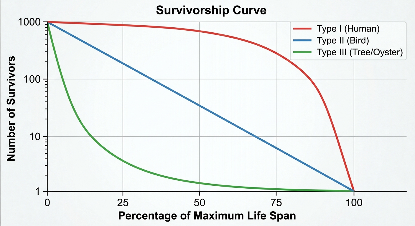
- Type I (Late Loss): Low death rates during early and middle life; death increases steeply in old age. (Humans/K-selected).
- Type II (Constant Loss): A constant death rate over the organism's life span (slope is straight). (Squirrels, some lizards).
- Type III (Early Loss): High death rates for the young; survivors flatten out and live a long time. (Oysters, insects/r-selected).
Population Demographics (Age Structure)
Age structure diagrams (population pyramids) show the relative number of individuals at each age. This helps predict future growth.
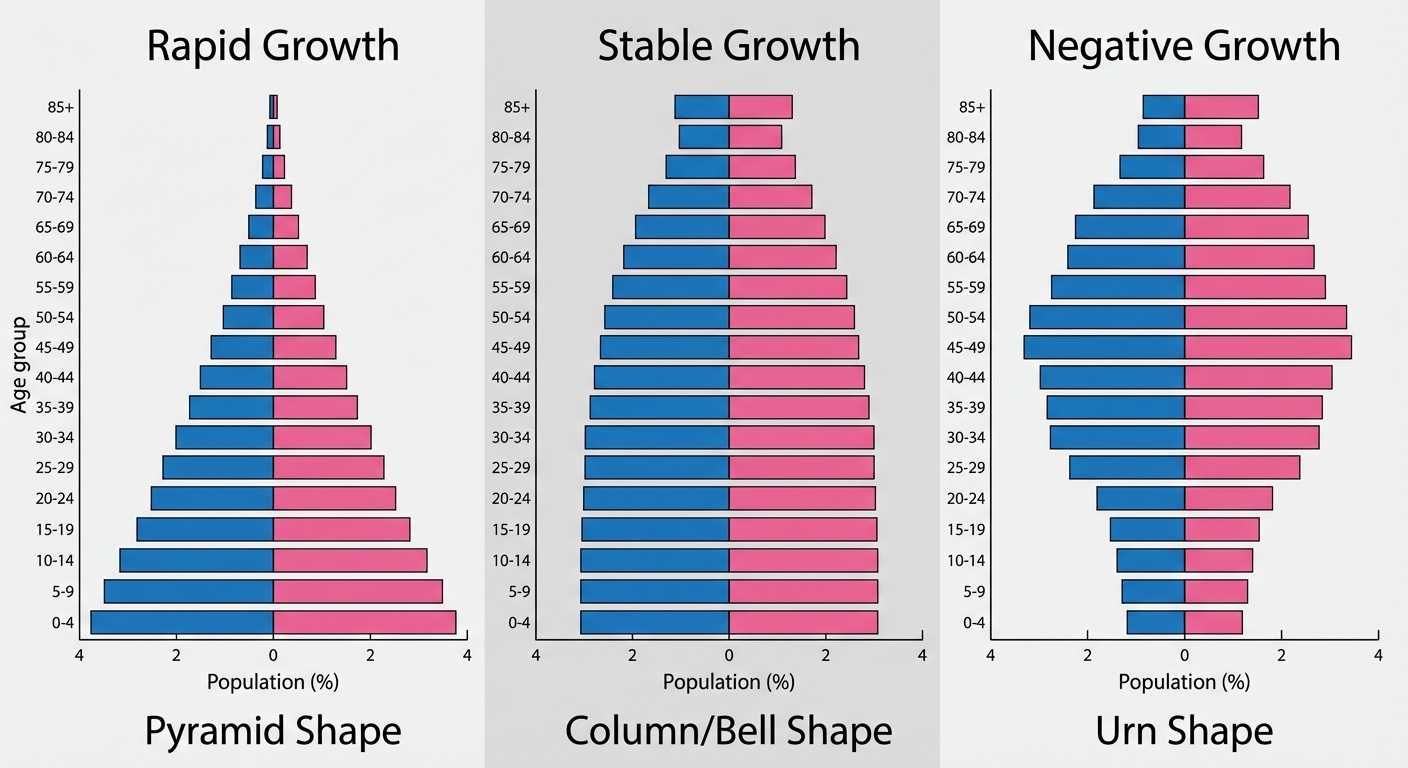
- Rapid Growth (Pyramid shape): Broad base. Massive number of young biological individuals who will soon reach reproductive age. (Example: Nigeria, Afghanistan).
- Stable Growth (Column shape): relatively even distribution among age groups. (Example: USA, Italy).
- Negative Growth (Inverted Pyramid): Narrow base. Fewer young people than older people. The population will shrink. (Example: Japan, Germany).
Common Mistakes & Pitfalls
Confusing Rate with Population Size
- Mistake: Thinking that if the growth rate ($dN/dt$) decreases, the population size ($N$) is decreasing.
- Correction: In Logistic growth, as you approach $K$, the rate slows down, but the population is still growing (adding individuals) until it hits zero growth. $N$ only decreases if $dN/dt$ is negative.
Carrying Capacity is NOT Static
- Mistake: Treating $K$ as a permanent, unchangeable number.
- Correction: Carrying capacity is a property of the environment using available resources. If the resource fluctuates (e.g., a drought reduces food), $K$ drops.
Misinterpreting "Maximum Growth" in Logistic Models
- Mistake: Assuming maximum growth occurs near $K$.
- Correction: In a logistic curve, the population grows fastest when $N$ is exactly half of $K$ ($K/2$). This is the inflection point of the sigmoid curve.
Mixing up Density Factors
- Mistake: Thinking a disease is density-independent because "viruses aren't alive."
- Correction: Disease transmission relies on proximity. The denser the population, the faster the spread. Therefore, disease is Density-Dependent.