Mastering Differential Equations: Separation of Variables
Understanding Separable Differential Equations
Definitions & Concepts
In AP Calculus AB, a major component of Unit 7 is solving differential equations algebraically. A differential equation is an equation involving a function and its derivative. The goal is to find the function $y = f(x)$ that satisfies the relationship.
Not all differential equations can be solved easily, but in this course, we focus on Separable Differential Equations. These are equations where the variables $x$ and $y$ can be algebraically separated onto opposite sides of the equation.
Formally, a differential equation is separable if it can be written in the form:
Here, the derivative is the product of a function of $x$ and a function of $y$. By dividing and multiplying, we can rearrange this into:
Once in this form, we can integrate both sides to find the solution.
General vs. Particular Solutions
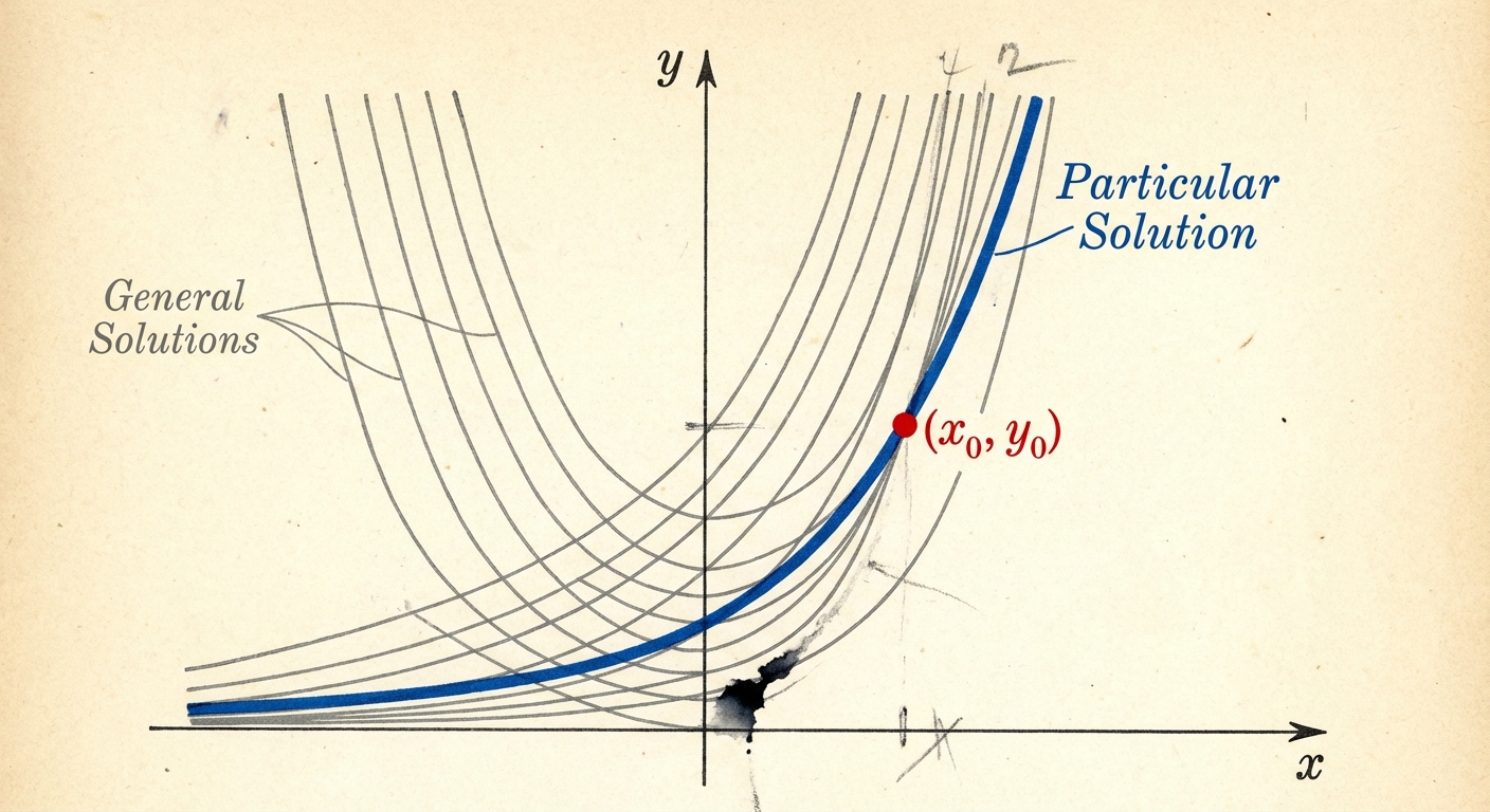
- General Solution: Represents a family of functions involving an arbitrary constant, $+C$. Graphically, this looks like many parallel or related curves (as seen in the image above).
- Particular Solution: A specific function derived from the general solution using an Initial Condition (e.g., $y(0) = 5$). This solution represents the single curve that passes through a specific point on the coordinate plane.
Finding General Solutions Using Separation of Variables
The Step-by-Step Algorithm
On the AP Exam Free Response Questions (FRQ), separating variables effectively accounts for the majority of points in differential equation problems. Follow this strict protocol:
- Separate: Algebraically move all terms involving $y$ (including $dy$) to one side and all terms involving $x$ (including $dx$) to the other.
- Integrate: Apply the integral symbol $\int$ to both sides. Find the antiderivative of each side independently.
- Add Constant: Add $+C$ to the side with the independent variable (usually $x$). Do not wait—add it immediately after integrating.
- Solve for y: Use algebra to isolate $y$. This typically involves exponentiation to remove natural logs or taking roots to remove powers.
Important Formulas & Integration Rules
When separating variables, you will frequently encounter these integration rules:
Power Rule (Reverse):
Logarithmic Rule (Key Concept):
Note: The absolute value bars are mandatory until determined otherwise by initial conditions.
Exponential Relationship:
If $\ln|y| = x + C$, then $|y| = e^{x+C}$. This simplifies to $y = Ae^x$ (where $A = \pm e^C$).
Worked Example: General Solution
Problem: Find the general solution for the differential equation $\frac{dy}{dx} = xy^2$.
Solution:
Separate: Divide by $y^2$ and multiply by $dx$.
Integrate:
Solve for y:
Multiply by -1:
Take the reciprocal:
(Note: Since $C$ is arbitrary, $-C$ is just another constant, often relabeled or left as $C$).
Finding Particular Solutions Using Initial Conditions
Finding the particular solution requires finding the specific value of $C$ that satisfies a given point $(x0, y0)$.
Procedure
- Perform the separation and integration steps as usual.
- Once you have the equation with $+C$, plug in the initial condition $x0$ and $y0$ immediately.
- Solve for $C$.
- Plug $C$ back into the equation and isolate $y$.
Worked Example: Particular Solution
Problem: Find the particular solution $y = f(x)$ to the differential equation $\frac{dy}{dx} = \frac{x}{y}$ with initial condition $f(0) = -2$.
Step 1: Separate Variables
Step 2: Integrate Both Sides
Step 3: Apply Initial Condition
Use $x = 0$ and $y = -2$ to solve for $C$.
So, the equation is:
Step 4: Solve for $y$
Multiply by 2:
Take the square root:
Crucial Step: Which sign do we choose? Look at the initial condition $f(0) = -2$. Since $y$ must be negative, we choose the negative branch.
Final Answer:
The Logic of Exponential Growth and Decay
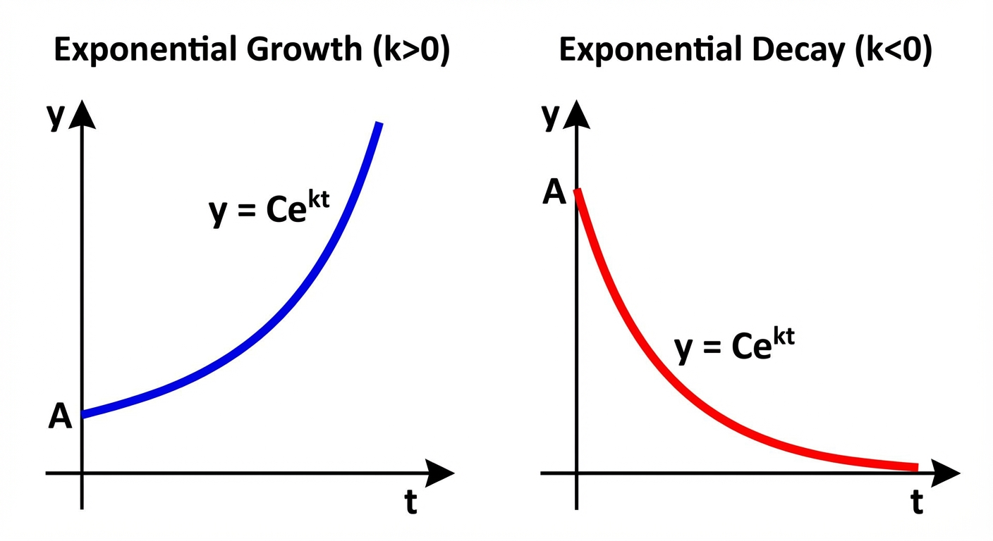
A very common pattern on the AP exam involves relationships where the rate of change is proportional to the amount present: $\frac{dy}{dt} = ky$.
When you separate this, you get:
Here, $A$ represents the initial value $y(0)$. This derivation is frequent enough that you should be comfortable reproducing it quickly.
Common Mistakes & Pitfalls
In the context of the AP Calculus AB exam, students frequently lose points on the following errors. Be vigilant!
1. The Separation Sin (0 Points)
If you do not algebraically separate $x$ and $y$ correctly (e.g., trying to subtract terms instead of dividing), you will receive zero points for the entire problem, even if your integration is correct later. Separation handles multiplication/division, not addition/subtraction.
- Wrong: $\frac{dy}{dx} = x + y \rightarrow dy - y = x dx$ (This is invalid).
2. Forgetting the Constant of Integration (+C)
If you forget $+C$, you cannot mathematically solve for the initial condition. On FRQs, if $+C$ is not present, you are usually capped at gaining only half the available points.
3. The Absolute Value Trap
When integrating $\int \frac{1}{y} dy$, you MUST write $\ln|y|$.
- If $y$ is positive based on the initial condition, the bars drop: $\ln(y)$.
- If $y$ is negative, the bars effectively negate $y$: $\ln(-y)$.
4. Improper Algebra with Logs
Remember log properties:
- $e^{a+b} \neq e^a + e^b$. It is $e^a \cdot e^b$.
- $e^{3\ln x} \neq 3x$. It is $e^{\ln x^3} = x^3$.
5. Domain of Validity
Sometimes a question asks for the "domain over which the solution is valid." The domain of a geometric series solution typically depends on the vertical asymptotes. A particular solution to a differential equation is only valid on the single continuous interval that contains the initial condition.