Unit 2 Study Guide: Market Dynamics and Policy Impacts
Unit 2: Supply and Demand — Market Equilibrium and Government Intervention
This section bridges the gap between theoretical curves and real-world market outcomes. We examine how markets naturally find stability and how government actions—like price controls, taxes, and trade tariffs—disrupt that stability, often leading to unintended consequences.
Market Equilibrium
Market Equilibrium occurs when the quantity of a good that consumers are willing and able to buy equals the quantity that producers are willing and able to sell. At this point, there is no tendency for the price to change unless an external factor shifts the curves.
- Equilibrium Price ($P_e$): The price at which quantity demanded equals quantity supplied.
- Equilibrium Quantity ($Q_e$): The quantity bought and sold at the equilibrium price.
Disequilibrium: Shortages and Surpluses
When the market price differs from $P_e$, disequilibrium occurs:
- Surplus (Excess Supply): Occurs when the market price is above equilibrium ($P > P_e$).
- $Qs > Qd$
- Market Correction: Producers lower prices to clear excess inventory, moving the market back toward equilibrium.
- Shortage (Excess Demand): Occurs when the market price is below equilibrium ($P < P_e$).
- $Qd > Qs$
- Market Correction: Consumers bid up prices for scarce goods, moving the market back toward equilibrium.
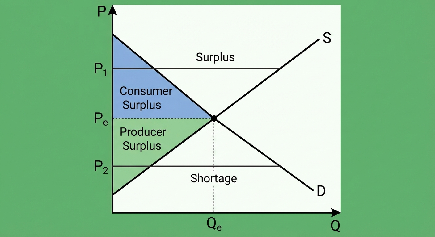
Consumer and Producer Surplus
These concepts measure the welfare or benefit that market participants receive.
Consumer Surplus (CS)
This is the difference between what a consumer is willing to pay (their maximum valuation) and what they actually pay (the market price).
- Graphically: The area below the Demand curve and above the Price line.
- Formula: Area of a Triangle $\rightarrow \frac{1}{2} \times \text{base} \times \text{height}$
Producer Surplus (PS)
This is the difference between the price a producer receives and the minimum price they were willing to accept (marginal cost).
- Graphically: The area above the Supply curve and below the Price line.
Total Surplus (Social Surplus)
When a market is in equilibrium without interference, Allocative Efficiency is achieved, meaning Total Surplus is maximized. There is no Deadweight Loss.
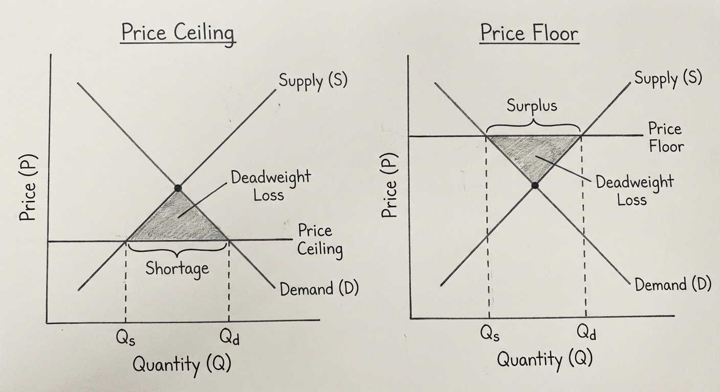
Price Ceilings and Floors
Governments sometimes mandate prices when they believe the equilibrium price is unfair. These controls prevent the market from clearing.
Price Ceilings
A Price Ceiling is a legal maximum on the price at which a good can be sold (e.g., rent control).
- Goal: Help consumers by keeping prices low.
- Binding vs. Non-Binding:
- To be effective (binding), a ceiling must be set BELOW the equilibrium price.
- If set above equilibrium, it has no effect (the market simply trades at equilibrium).
- Consequences of Binding Ceilings:
- Shortage: $Qd > Qs$.
- Deadweight Loss: Quantity sold decreases to $Q_s$. Mutually beneficial transactions are prevented.
- Inefficient Allocation: Goods may not go to consumers who value them most.
- Black Markets: Illegal trading at higher prices.
Price Floors
A Price Floor is a legal minimum on the price at which a good can be sold (e.g., minimum wage, agricultural supports).
- Goal: Help producers (or workers) by keeping prices (or wages) high.
- Binding vs. Non-Binding:
- To be effective (binding), a floor must be set ABOVE the equilibrium price.
- If set below equilibrium, it has no effect.
- Consequences of Binding Floors:
- Surplus: $Qs > Qd$.
- Deadweight Loss: Quantity bought decreases to $Q_d$.
Memory Aid: To represent a restriction on the room you are in: The Ceiling is below you (crouching down/shortage), and the Floor is above you (floating up/surplus). It sounds backward, but remember: A binding ceiling is below the top ($Pe$), and a binding floor is above the bottom ($Pe$).
Taxes and Subsidies
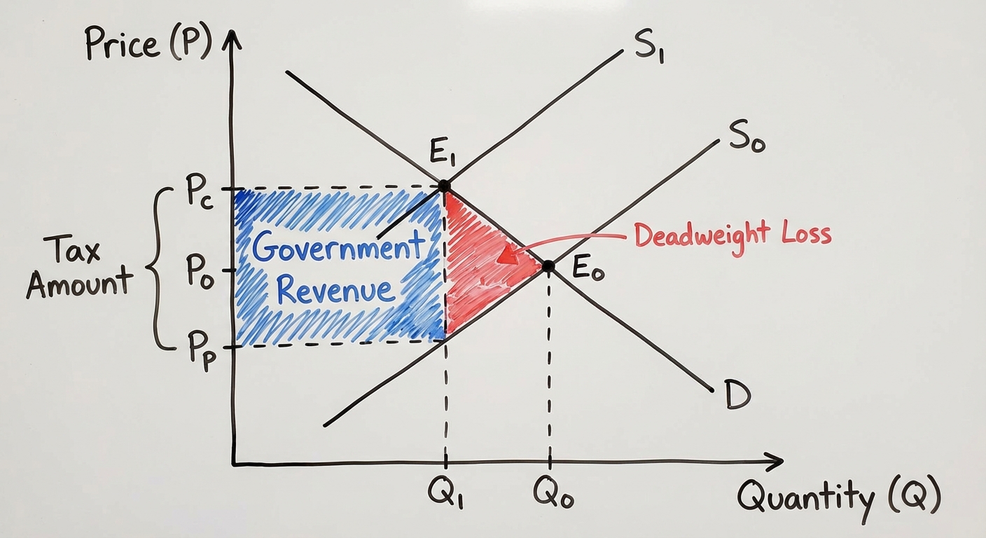
Excise Taxes
An Excise Tax is a per-unit tax on a specific good (e.g., gasoline, cigarettes).
- The Shift: Graphically, this shifts the Supply curve vertically upward by the amount of the tax.
- Tax Wedge: The vertical distance between the $S$ and $S{tax}$ curves at the new quantity ($Qt$).
- Prices:
- $P_c$ (Price Consumers Pay): Increases.
- $Pp$ (Price Producers Keep): Decreases ($Pp = P_c - \text{TaxAmount}$).
- Tax incidence: Who actually pays the tax? It depends on Elasticity.
- If Demand is generally inelastic relative to Supply, consumers bear more of the burden.
- If Supply is generally inelastic relative to Demand, producers bear more of the burden.
Calculating Outcomes
- Tax Revenue:
- Deadweight Loss (DWL): The loss of total surplus resulting from the tax reducing the market quantity.
Subsidies
A Subsidy is a government payment that supports a business or market. It is essentially a "negative tax."
- Shift: Supply shifts right/down.
- Outcome: Quantity increases, price to consumers falls, price received by producers rises. However, it still creates Deadweight Loss because it encourages over-production (producing units that cost more to make than consumers value them).
International Trade and Tariffs
When a country opens to the world market (Autarky $\rightarrow$ Free Trade), the domestic price adjusts to the World Price ($P_W$).
Importing vs. Exporting
- If $PW < P{Domestic}$: The country has a comparative disadvantage. They will Import. Domestic $Qs$ falls, Domestic $Qd$ rises. Consumers win; Producers lose.
- If $PW > P{Domestic}$: The country has a comparative advantage. They will Export. Domestic $Qs$ rises, Domestic $Qd$ falls. Producers win; Consumers lose.
Tariffs
A Tariff is a tax on imported goods.
- Mechanism: It raises the effective price of imports from $PW$ to $PW + \text{Tariff}$.
- Effects:
- Domestic production increases ($Q_s$ rises).
- Domestic consumption decreases ($Q_d$ falls).
- Imports decrease.
- Government Revenue is generated.
- Deadweight Loss is created (inefficiency from over-producing domestically and under-consuming).
Common Mistakes & Pitfalls
- Confusing Binding vs. Non-Binding:
- Mistake: Thinking a price ceiling means the price goes "up to the ceiling."
- Correction: A binding ceiling prevents the price from going up to equilibrium. It must be low.
- Misidentifying Tax Incidence:
- Mistake: Thinking the statutory payer (who writes the check) bears the burden.
- Correction: The burden is always shared based on elasticity, regardless of who the law targets.
- Deadweight Loss Location:
- Mistake: Placing DWL randomly.
- Correction: DWL is always a triangle pointing toward the equilibrium point ($Pe, Qe$). It represents the trades that didn't happen (or shouldn't have happened, in the case of subsidies).
- Double Counting Surplus:
- Mistake: Including Tax Revenue in Deadweight Loss.
- Correction: Total Welfare under tax = Consumer Surplus + Producer Surplus + Tax Revenue. The DWL is the surplus that simply vanished.