AP Calculus AB Unit 1 Study Guide: Limits, Continuity, Asymptotes, and the IVT

What a limit means (and why calculus starts here)

A limit describes what value a function is approaching as the input gets close to a particular number. The key idea is that limits are about nearby behavior, not necessarily what happens exactly at the point. That “nearby” focus is what makes limits powerful: they let you talk precisely about change, motion, and trend even when a function has a hole, a jump, or grows without bound.

In everyday language, when you say “as $x$ gets close to $a$, $f(x)$ gets close to $L$,” you’re describing a limit. In calculus notation, that statement is written as:

$\lim_{x \to a} f(x) = L$

This reads: “the limit of $f(x)$ as $x$ approaches $a$ equals $L$.”

A practical starting point: to find the limit of a simple polynomial, you can usually plug in the number that the variable is approaching.

Approaching vs. arriving

A common early confusion is mixing up the limit with the actual function value. The limit cares about values of $f(x)$ when $x$ is **close to** $a$ (like $a - 0.001$ or $a + 0.001$), not necessarily at $x = a$.

That’s why it’s possible for a limit to exist even if:

• $f(a)$ is undefined (there’s a hole), or
• $f(a)$ is defined but not equal to the limit (a “redefined point”), or
• $f(x)$ has a jump or vertical asymptote at $a$ (then the limit might not exist or might be infinite).

Two-sided limits and one-sided limits

A two-sided limit checks what happens as you approach from both sides:

$\lim_{x \to a} f(x) = L$

A one-sided limit checks only one direction:

$\lim_{x \to a^-} f(x) = L$

$\lim_{x \to a^+} f(x) = L$

Here, $a^-$ means approaching $a$ from values _less than_ $a$ (the left), and $a^+$ means approaching $a$ from values _greater than_ $a$ (the right).

The crucial relationship is that

$\lim_{x \to a} f(x) = L$

exists (and equals $L$) if and only if both one-sided limits exist and are equal to the same number:

$\lim_{x \to a^-} f(x) = \lim_{x \to a^+} f(x) = L$

If the left-hand and right-hand limits don’t match, the two-sided limit does not exist.

Ways to find limits (the main toolkit)

In this unit you’ll repeatedly evaluate limits in four main ways:

• Look on a graph to see what value the function approaches.
• If the graph approaches two different values from the left and right for the same input, the (two-sided) limit does not exist.
• Estimate from a table by checking values close to the target from both sides.
• Use algebra (limit laws and simplification) to compute exact limits.

Limit notation you’ll see on AP

You’ll encounter multiple notations that mean the same idea. Here’s a quick reference:

Why limits matter in calculus

Limits are the foundation for two major ideas you’ll build soon:

1. Derivatives: the instantaneous rate of change is defined using a limit of average rates of change.
2. Integrals: area accumulation is defined using a limit of sums.

So when you learn to evaluate limits and interpret them correctly, you’re learning the language calculus uses to define its main tools.

Worked example 1: limit vs. function value

Suppose a function is defined by:

$f(x) = \frac{x^2 - 1}{x - 1}$

If you plug in $x = 1$, you get $\frac{0}{0}$, which is undefined—so $f(1)$ does not exist (there’s a hole). But you can still ask what value the function approaches as $x$ gets close to $1$.

Factor the numerator:

$x^2 - 1 = (x - 1)(x + 1)$

So for $x \ne 1$:

$f(x) = \frac{(x - 1)(x + 1)}{x - 1} = x + 1$

Now it’s clear that as $x \to 1$, $f(x)$ approaches $2$:

$\lim_{x \to 1} \frac{x^2 - 1}{x - 1} = 2$

Important takeaway: a limit can exist even when the function is not defined at that point.

Worked example 2: when a two-sided limit does not exist

Define a function by pieces: $g(x)=1$ for $x<0$ and $g(x)=3$ for $x \ge 0$.

Approach $0$ from the left: values are constantly $1$, so:

$\lim_{x \to 0^-} g(x) = 1$

Approach $0$ from the right: values are constantly $3$, so:

$\lim_{x \to 0^+} g(x) = 3$

Since the one-sided limits are not equal, the two-sided limit does not exist:

$\lim_{x \to 0} g(x) \text{ does not exist}$

Exam Focus

• Typical question patterns:
  • “Evaluate $\lim_{x \to a} f(x)$ from a graph/table and justify your answer.”
  • “Find $\lim_{x \to a^-} f(x)$ and $\lim_{x \to a^+} f(x)$, then determine whether $\lim_{x \to a} f(x)$ exists.”
  • “Explain the difference between $f(a)$ and $\lim_{x \to a} f(x)$.”
• Common mistakes:
  • Plugging in $x = a$ automatically and assuming that gives the limit (this fails at holes and jumps).
  • Forgetting that two-sided limits require both one-sided limits to agree.
  • Using the function value at the point to decide the limit (limits depend on nearby values, not the point).

Estimating limits from graphs and tables

Before using algebra, you need to be able to read limits from representations. AP questions often give you a graph or a table and ask for limits, one-sided limits, or whether a limit exists. The skill is really about careful interpretation: you’re looking for the y-values the function approaches as $x$ approaches a target.

Reading limits from graphs

When a graph is provided, you estimate:

• Approach $a$ from the left and trace the curve to see what y-value it heads toward.
• Approach $a$ from the right and do the same.
• Decide whether those two y-values match.

A few common graph features matter a lot:

• An open circle indicates the function is not defined at that exact point (or not taking that value there), but it still shows what the graph approaches.
• A filled dot gives the actual value $f(a)$.
• A vertical asymptote suggests the function grows without bound near that $x$-value.

What tables can and cannot tell you

A table of values can suggest a limit by showing values of $f(x)$ for $x$ close to $a$. But tables come with a warning: you’re inferring a trend from finite data.

To use tables well:

• Look at values approaching $a$ from both sides.
• Watch whether $f(x)$ appears to settle toward one number.
• Be cautious if values change rapidly or seem to head off to very large magnitudes.

Also, a table can’t prove a limit exists, but on AP it’s often sufficient to make a reasonable estimate (and sometimes you’ll be asked to justify with the pattern shown).

Example 1: estimating from a table

Suppose you’re given values near $x = 2$:

The values approach $5$ as $x$ approaches $2$ from both sides, so you would estimate:

$\lim_{x \to 2} f(x) = 5$

Notice you didn’t need to know $f(2)$.

Example 2: one-sided limit from a graph description

Imagine a graph where as $x$ approaches $1$ from the left, the curve approaches height $2$, but as $x$ approaches $1$ from the right, the curve approaches height $-1$. Then:

$\lim_{x \to 1^-} f(x) = 2$

$\lim_{x \to 1^+} f(x) = -1$

So:

$\lim_{x \to 1} f(x) \text{ does not exist}$

A useful mental picture: “zooming in”

A good way to understand limits graphically is to imagine zooming in on the graph near $x = a$. If, after zooming in, the curve approaches a single height from both sides, the limit exists and equals that height—even if there’s a hole or a misplaced point.

Exam Focus

• Typical question patterns:
  • “Use the graph to determine $\lim_{x \to a} f(x)$ and $f(a)$.”
  • “Given a table, estimate the limit and state whether it appears to be finite or infinite.”
  • “Determine whether $\lim_{x \to a} f(x)$ exists; if not, explain using one-sided limits.”
• Common mistakes:
  • Reading the filled dot as the limit when the curve approaches a different y-value.
  • Ignoring direction in one-sided limits (mixing up left and right).
  • Using table values too far from $a$ and missing the local trend.

Evaluating limits algebraically with limit laws

Graph and table estimates are useful, but algebra is how you compute exact limits reliably. The big idea is that for many functions, you can “substitute” $x = a$ into the formula to find the limit—as long as the function behaves nicely there.

Direct substitution (when it works)

If $f(x)$ is a polynomial, a rational function with nonzero denominator at $a$, or a combination of continuous functions, then:

$\lim_{x \to a} f(x) = f(a)$

This is not a random trick—it’s a consequence of continuity. For now, think: if there’s no hole, jump, or asymptote at $a$, then approaching $a$ should give the same value as plugging in $a$.

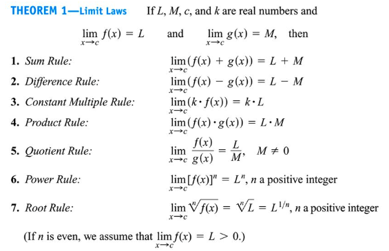
Limit laws (the “legal moves”)

Limit laws let you break complicated limits into simpler ones. Suppose:

$\lim_{x \to a} f(x) = L$

and

$\lim_{x \to a} g(x) = M$

Then (when the limits on the right exist and denominators are not zero):

$\lim_{x \to a} (f(x) + g(x)) = L + M$

$\lim_{x \to a} (f(x) - g(x)) = L - M$

$\lim_{x \to a} (c f(x)) = cL$

$\lim_{x \to a} (f(x) g(x)) = LM$

$\lim_{x \to a} \frac{f(x)}{g(x)} = \frac{L}{M}$

A common AP-style reference chart for these algebraic properties looks like this:

The big warning sign: indeterminate forms

A common situation in algebraic limits is that direct substitution gives:

$\frac{0}{0}$

This is called an indeterminate form. It does not mean the limit is zero or undefined—it means “the algebra hasn’t told you the answer yet.” Usually, you must simplify the expression to reveal the underlying behavior.

The most common AP Calculus AB strategies for $\frac{0}{0}$ are:

• factoring and canceling a common factor,
• using a common denominator,
• rationalizing with a conjugate.

Strategy 1: factoring and canceling (removable discontinuities)

This is mostly useful if you get limits where the denominator is equal to $0$ after substitution, creating a hole-type issue (a removable discontinuity). You factor the numerator and denominator, then cancel any common factor.

A quick illustration of the idea (showing what can be removed):

$\frac{(x+3)(x+2)}{(x+3)(x-3)}$

The factor $x+3$ is common to top and bottom, so it is able to be removed. That cancellation corresponds to a **removable discontinuity** at the input value that makes $x+3=0$.

Example 1

Evaluate:

$\lim_{x \to 3} \frac{x^2 - 9}{x - 3}$

Direct substitution gives $\frac{0}{0}$, so factor:

$x^2 - 9 = (x - 3)(x + 3)$

For $x \ne 3$:

$\frac{x^2 - 9}{x - 3} = \frac{(x - 3)(x + 3)}{x - 3} = x + 3$

Now take the limit:

$\lim_{x \to 3} (x + 3) = 6$

Conceptually, you removed the “hole-causing factor,” then evaluated what the function is approaching.

Strategy 2: common denominators (complex rational expressions)

Sometimes the expression has smaller fractions inside it. The goal is to combine terms so you can simplify.

Example 2

Evaluate:

$\lim_{x \to 1} \frac{\frac{1}{x} - 1}{x - 1}$

First simplify the numerator:

$\frac{1}{x} - 1 = \frac{1 - x}{x}$

So the expression becomes:

$\frac{\frac{1 - x}{x}}{x - 1} = \frac{1 - x}{x(x - 1)}$

Notice $1 - x = -(x - 1)$:

$\frac{1 - x}{x(x - 1)} = \frac{-(x - 1)}{x(x - 1)} = -\frac{1}{x}$

Now evaluate the limit:

$\lim_{x \to 1} -\frac{1}{x} = -1$

Strategy 3: rationalizing with a conjugate

This is common when you have square roots. The conjugate helps eliminate radicals and expose a cancelable factor.

Example 3

Evaluate:

$\lim_{x \to 0} \frac{\sqrt{x + 9} - 3}{x}$

Direct substitution gives $\frac{0}{0}$. Multiply numerator and denominator by the conjugate:

$\frac{\sqrt{x + 9} - 3}{x} \cdot \frac{\sqrt{x + 9} + 3}{\sqrt{x + 9} + 3}$

The numerator becomes a difference of squares:

$({\sqrt{x + 9}})^2 - 3^2 = (x + 9) - 9 = x$

So the expression simplifies to:

$\frac{x}{x(\sqrt{x + 9} + 3)} = \frac{1}{\sqrt{x + 9} + 3}$

Now substitute $x = 0$:

$\frac{1}{\sqrt{9} + 3} = \frac{1}{6}$

Piecewise functions and limits

With a piecewise function, the limit at the “break point” often depends on matching behavior from both sides.

Example 4

Let $f(x)=x^2-1$ for $x<1$ and $f(x)=2x+k$ for $x \ge 1$. Find $k$ so that $\lim_{x \to 1} f(x)$ exists.

Compute the one-sided limits.

Left-hand limit (use the first piece):

$\lim_{x \to 1^-} (x^2 - 1) = 1^2 - 1 = 0$

Right-hand limit (use the second piece):

$\lim_{x \to 1^+} (2x + k) = 2(1) + k = 2 + k$

For the two-sided limit to exist, set them equal:

$0 = 2 + k$

So:

$k = -2$

Exam Focus

• Typical question patterns:
  • “Evaluate the limit; if direct substitution gives $\frac{0}{0}$, algebraically simplify.”
  • “Find a parameter value so a limit exists (or so left and right limits match).”
  • “Compute one-sided limits of a piecewise function at a boundary point.”
• Common mistakes:
  • Treating $\frac{0}{0}$ as an answer instead of a signal to simplify.
  • Canceling terms that are not factors (you may only cancel common factors, not terms across addition).
  • Using the wrong piece of a piecewise function when approaching from the left or right.

Key limit theorems and special techniques (including Squeeze)

Some limits aren’t best handled by algebraic simplification alone. In Unit 1, two ideas come up repeatedly: using known “parent” limits (especially with trigonometric expressions), and using bounds to trap a function’s limit.

The Squeeze Theorem (pinching a limit)

The Squeeze Theorem formalizes a simple idea: if a function is trapped between two other functions that approach the same limit, then the trapped function must approach that limit too.

Suppose for $x$ near $a$ you have:

$g(x) \le f(x) \le h(x)$

and

$\lim_{x \to a} g(x) = \lim_{x \to a} h(x) = L$

Then:

$\lim_{x \to a} f(x) = L$

Why it matters: this is one of the few tools that lets you evaluate limits when simplification is difficult but you can establish good inequalities.

Example 1: a classic squeeze limit

Evaluate:

$\lim_{x \to 0} x^2 \sin\left(\frac{1}{x}\right)$

This is tricky because $\sin\left(\frac{1}{x}\right)$ oscillates infinitely often near $0$, so direct substitution doesn’t help.

But you know for any input $u$:

$-1 \le \sin(u) \le 1$

So:

$-1 \le \sin\left(\frac{1}{x}\right) \le 1$

Multiply all parts by $x^2$. Since $x^2 \ge 0$, the inequality directions do not change:

$-x^2 \le x^2 \sin\left(\frac{1}{x}\right) \le x^2$

Now take limits as $x \to 0$:

$\lim_{x \to 0} (-x^2) = 0$

$\lim_{x \to 0} x^2 = 0$

So the middle function is squeezed to $0$:

$\lim_{x \to 0} x^2 \sin\left(\frac{1}{x}\right) = 0$

A common misconception is thinking “since sine oscillates, the limit doesn’t exist.” Oscillation alone doesn’t prevent a limit—if the oscillation amplitude shrinks to zero, the limit can exist.

Special trigonometric limits you should know

AP Calculus AB expects you to use certain standard trigonometric limit results. The most central one is:

$\lim_{x \to 0} \frac{\sin(x)}{x} = 1$

This limit is foundational because it powers many other trig limits through algebraic manipulation.

Closely related results include:

$\lim_{x \to 0} \frac{\tan(x)}{x} = 1$

$\lim_{x \to 0} \frac{1 - \cos(x)}{x} = 0$

and, written equivalently,

$\lim_{x \to 0} \frac{\cos(x) - 1}{x} = 0$

Two especially useful “parameter” forms are:

$\lim_{x \to 0} \frac{\sin(ax)}{x} = a$

$\lim_{x \to 0} \frac{\sin(ax)}{\sin(bx)} = \frac{a}{b}$

Using substitution with trig limits

If you see something like $\sin(5x)$, you want the inside to look like “something going to 0.” Let $u = 5x$. As $x \to 0$, $u \to 0$.

Example 2

Evaluate:

$\lim_{x \to 0} \frac{\sin(5x)}{x}$

Rewrite to create the standard form:

$\frac{\sin(5x)}{x} = \frac{\sin(5x)}{5x} \cdot 5$

Now apply the known limit:

$\lim_{x \to 0} \frac{\sin(5x)}{5x} = 1$

So:

$\lim_{x \to 0} \frac{\sin(5x)}{x} = 5$

Example 3

Evaluate:

$\lim_{x \to 0} \frac{\tan(3x)}{x}$

Rewrite similarly:

$\frac{\tan(3x)}{x} = \frac{\tan(3x)}{3x} \cdot 3$

Then:

$\lim_{x \to 0} \frac{\tan(3x)}{3x} = 1$

So:

$\lim_{x \to 0} \frac{\tan(3x)}{x} = 3$

A note about angles (radians)

Those standard trig limits are true when angles are measured in radians. In AP Calculus, radian mode is assumed essentially everywhere. If you used degrees, these limits would not evaluate to the same values.

Exam Focus

• Typical question patterns:
  • “Evaluate a limit using the Squeeze Theorem; justify the inequalities used.”
  • “Compute a trig limit by rewriting into the form $\frac{\sin(u)}{u}$ or $\frac{\tan(u)}{u}$.”
  • “Decide whether an oscillating function has a limit near a point.”
• Common mistakes:
  • Forgetting to rewrite expressions to match the known trig limit forms (especially missing the factor adjustment).
  • Assuming oscillation automatically means ‘limit does not exist’ without checking whether the oscillation is being damped.
  • Working in degrees conceptually (AP calculus trig limits rely on radian measure).

Limits involving infinity: end behavior and infinite limits

Limits don’t only describe behavior near a finite point $a$. They also describe what happens as $x$ becomes very large in magnitude, and what happens when a function grows without bound near a point. These ideas connect directly to asymptotes and to understanding long-run behavior.

Limits as $x$ approaches infinity

A limit like:

$\lim_{x \to \infty} f(x) = L$

means that as $x$ becomes larger and larger, $f(x)$ gets closer and closer to $L$.

If this limit exists and equals a finite number $L$, then the line:

$y = L$

is a horizontal asymptote of the function (describing end behavior). A horizontal asymptote describes end behavior and can be crossed by the graph.

Similarly:

$\lim_{x \to -\infty} f(x) = L$

describes the left-end behavior.

Infinite limits, vertical asymptotes, and “cannot cross”

Sometimes a function does not approach a finite value as $x$ approaches a number $a$. Instead, the function may increase or decrease without bound. For example:

$\lim_{x \to a} f(x) = \infty$

means $f(x)$ grows arbitrarily large near $a$.

This often corresponds to a vertical asymptote at:

$x = a$

A vertical asymptote is a line where the function is undefined; in typical rational-function graphs, it’s a line the function cannot cross because the function has no defined value there.

Direction matters—one side could go to $\infty$ while the other goes to $-\infty$.

Example 3

Evaluate one-sided behavior:

$f(x) = \frac{1}{x - 2}$

As $x \to 2^+$, the denominator is a small positive number, so the fraction becomes very large positive:

$\lim_{x \to 2^+} \frac{1}{x - 2} = \infty$

As $x \to 2^-$, the denominator is a small negative number, so the fraction becomes very large negative:

$\lim_{x \to 2^-} \frac{1}{x - 2} = -\infty$

Because the one-sided limits are not equal (and not finite), the two-sided limit does not exist. But it’s still meaningful to describe the infinite one-sided limits.

Evaluating limits at infinity for rational functions (horizontal asymptote rules)

For rational functions (ratios of polynomials), end behavior is controlled mainly by the highest power of $x$ in the numerator and denominator.

Let:

$f(x) = \frac{a_n x^n + \text{lower powers}}{b_m x^m + \text{lower powers}}$

Compare degrees $n$ and $m$:

• If $n < m$, then:

$\lim_{x \to \infty} f(x) = 0$

So the horizontal asymptote is $y=0$.

• If $n = m$, then:

$\lim_{x \to \infty} f(x) = \frac{a_n}{b_m}$

So the horizontal asymptote is $y=\frac{a_n}{b_m}$.

• If $n > m$, the function does **not** approach a finite constant. In many such cases the values grow without bound (often described informally as “the limit as $x$ approaches infinity is infinity”), and there is no horizontal asymptote (though there may be a slant/oblique asymptote in later units).

Example 1 (numerator degree smaller)

Evaluate:

$\lim_{x \to \infty} \frac{3x + 1}{x^2 + 4}$

Degree numerator is $1$, degree denominator is $2$, so the denominator grows faster. The limit is:

$0$

So $y = 0$ is a horizontal asymptote.

Example 2 (same degree)

Evaluate:

$\lim_{x \to \infty} \frac{5x^2 - x}{2x^2 + 7}$

Same degree, so take the ratio of leading coefficients:

$\frac{5}{2}$

So $y = \frac{5}{2}$ is a horizontal asymptote.

Distinguishing “does not exist” from “infinite”

On AP, be careful with language:

• If you mean the function grows without bound, you should write $\infty$ or $-\infty$ as the limit (that’s an infinite limit).
• If left and right behaviors disagree, you should say the two-sided limit does not exist.

For example, for $\frac{1}{x - 2}$, the two-sided limit at $2$ does not exist, even though each one-sided limit is infinite.

Exam Focus

• Typical question patterns:
  • “Find the horizontal asymptote by computing $\lim_{x \to \infty} f(x)$.”
  • “Determine vertical asymptotes and infinite one-sided limits from a formula or graph.”
  • “Compare $\lim_{x \to \infty} f(x)$ and $\lim_{x \to -\infty} f(x)$ (they may differ).”
• Common mistakes:
  • Saying a limit ‘does not exist’ when it actually is $\infty$ or $-\infty$ (or vice versa).
  • Forgetting to check one-sided behavior near vertical asymptotes.
  • Mishandling degree comparisons for rational functions (especially ignoring leading coefficients).

Continuity: connecting limits to function behavior

Continuity is the idea that a function’s graph has no breaks—informally, you can draw it without lifting your pencil (at least near the point you care about). In calculus, continuity is defined using limits, so this topic is really where the unit’s ideas tie together.

Continuity at a point

A function $f$ is **continuous at** $x = a$ if three conditions are met:

1. $f(a)$ is defined.
2. $\lim_{x \to a} f(x)$ exists.
3. $\lim_{x \to a} f(x) = f(a)$.

These conditions capture exactly what “no break at $a$” means: the function has a value there, approaching from both sides leads to a single value, and that approached value matches the function’s actual value.

Continuity on an interval

A function is continuous on an interval if it’s continuous at every point in that interval. When you work with intervals, endpoints require one-sided continuity (because you can only approach from inside the interval).

For example, continuous on $[a,b]$ means:

• continuous for $a < x < b$,
• right-continuous at $x = a$,
• left-continuous at $x = b$.

Types of discontinuities (how continuity can fail)

If a function is not continuous at $x = a$, it has a discontinuity there. In AP Calculus AB, the most common types are:

Removable discontinuity (a “hole”)

A removable discontinuity happens when the limit exists, but the function value is missing or doesn’t match.

Typical pattern:

• $\lim_{x \to a} f(x) = L$ exists,
• but $f(a)$ is undefined, or $f(a) \ne L$.

This is “removable” because you could make the function continuous by redefining $f(a)$ to equal the limit. Often you reveal this hole by factoring out a common factor in a rational expression.

Example idea: the function

$\frac{x^2 - 1}{x - 1}$

has a removable discontinuity at $x = 1$.

Jump discontinuity

A jump discontinuity occurs when the curve “breaks” at a particular place and starts somewhere else. The left-hand and right-hand limits are both finite but not equal:

$\lim_{x \to a^-} f(x) \ne \lim_{x \to a^+} f(x)$

So the two-sided limit does not exist. Graphically, the function “jumps” from one height to another.

Essential/infinite discontinuity (vertical asymptote)

An essential/infinite discontinuity occurs when the curve has a vertical asymptote and the function grows without bound near a point—at least one of the one-sided limits is $\infty$ or $-\infty$.

Continuity of common function types

It helps to know which functions are continuous “by default,” because then limits become easier:

• Polynomials are continuous for all real numbers.
• Rational functions are continuous wherever the denominator is not zero.
• Exponential, logarithmic (where defined), and trig functions are continuous on their domains.

This matters because it justifies direct substitution: if you know the function is continuous at $a$, then:

$\lim_{x \to a} f(x) = f(a)$

Removing discontinuities (redefining a function to fill a hole)

You can remove a discontinuity by redefining the function so that the “problem point” is handled differently (often by filling in the hole with the limit value). A very common case is a rational expression where factoring and canceling reveals the simplified expression; then you define the function at the excluded input to match the limit.

Example 1: checking continuity at a point

Determine whether $f(x)$ is continuous at $x = 2$ for a piecewise-defined function with:

• $f(x)=x^2-4$ for $x<2$,
• $f(2)=3$,
• $f(x)=x-2$ for $x>2$.

Step 1: compute left-hand limit:

$\lim_{x \to 2^-} (x^2 - 4) = 4 - 4 = 0$

Step 2: compute right-hand limit:

$\lim_{x \to 2^+} (x - 2) = 0$

So the two-sided limit exists and equals $0$:

$\lim_{x \to 2} f(x) = 0$

Step 3: compare to the function value:

$f(2) = 3$

Since $\lim_{x \to 2} f(x) \ne f(2)$, the function is **not continuous** at $x = 2$. This is a removable-type situation because the limit exists, but the function value has been set differently.

Example 2: making a function continuous by choosing a parameter

Let a function be defined by:

• $f(x)=\frac{x^2 - 1}{x - 1}$ for $x \ne 1$,
• $f(1)=k$.

Find $k$ so that $f$ is continuous at $x = 1$.

Continuity requires:

$k = f(1) = \lim_{x \to 1} \frac{x^2 - 1}{x - 1}$

From earlier simplification, for $x \ne 1$ the expression equals $x + 1$, so:

$\lim_{x \to 1} \frac{x^2 - 1}{x - 1} = 2$

Therefore:

$k = 2$

This kind of problem is very common: use a limit to fill in a hole.

Exam Focus

• Typical question patterns:
  • “Is $f$ continuous at $x = a$? Show the three continuity conditions.”
  • “Find a value of a parameter that makes a piecewise function continuous at a boundary.”
  • “Classify the discontinuity (removable, jump, infinite) using limits.”
• Common mistakes:
  • Checking only that $f(a)$ exists and forgetting to check whether the limit exists and matches.
  • Assuming a function is continuous at a point just because it’s defined there.
  • Mixing up removable vs. jump: if left and right limits differ, it’s not removable.

The Intermediate Value Theorem (IVT): why continuity guarantees solutions

The Intermediate Value Theorem (IVT) is one of the most important conceptual payoffs of continuity. It tells you that continuous functions can’t “skip” output values.

The theorem (what it says)

If $f$ is continuous on the closed interval $[a,b]$, and $N$ is any number between $f(a)$ and $f(b)$, then there exists at least one number $c$ in $[a,b]$ such that:

$f(c) = N$

In plain language: if you start at $f(a)$ and move continuously to $f(b)$, you must pass through every y-value in between.

Why IVT matters

IVT is a guarantee of existence. It does not necessarily tell you what $c$ is, but it tells you that a solution must be there.

This is powerful for:

• proving that an equation $f(x) = N$ has a solution,
• justifying that a root exists (a place where $f(x) = 0$),
• interpreting graphs and real-world models: if a continuous quantity changes from below a target value to above it, it must equal the target somewhere in between.

A real-world analogy: if the temperature (modeled continuously) goes from $60$ degrees at noon to $80$ degrees at 3 pm, then at some time between noon and 3 pm it must have been exactly $70$ degrees.

IVT requires continuity on the entire interval

A subtle but essential detail is that IVT requires $f$ to be continuous on **all of** $[a,b]$, not just at one point.

If there’s a discontinuity in the interval, the function can skip values by jumping.

Example 1: proving a root exists

Show that the equation:

$x^3 - 4x - 1 = 0$

has a solution in the interval $[1,2]$.

Let:

$f(x) = x^3 - 4x - 1$

This is a polynomial, so it is continuous everywhere, including on $[1,2]$.

Compute endpoints:

$f(1) = 1 - 4 - 1 = -4$

$f(2) = 8 - 8 - 1 = -1$

Both are negative, so IVT does not yet guarantee a root between them (you have not shown a sign change).

Try a different interval, say $[2,3]$:

$f(2) = -1$

$f(3) = 27 - 12 - 1 = 14$

Now $f(2) < 0$ and $f(3) > 0$. Since $0$ is between $-1$ and $14$, IVT guarantees there exists some $c$ in $[2,3]$ such that:

$f(c) = 0$

So the equation has at least one solution in $[2,3]$.

Notice what you proved: existence, not the exact value.

Example 2: IVT with a target value

Suppose $f$ is continuous on $[0,5]$, with $f(0) = 10$ and $f(5) = 2$. Prove there is a number $c$ in $[0,5]$ such that $f(c) = 6$.

Because $6$ is between $10$ and $2$, IVT applies and guarantees some $c$ exists with that output.

What IVT does not guarantee

Two common misunderstandings:

1. IVT does not guarantee uniqueness. There could be multiple values of $c$.
2. IVT does not apply without continuity. If the function has a jump, it can skip over values.

Exam Focus

• Typical question patterns:
  • “Use IVT to show there is a solution to $f(x) = 0$ in an interval; justify continuity and show the target lies between endpoint values.”
  • “Given a context (temperature, position, profit), argue a certain value must occur.”
  • “Explain why IVT cannot be applied (identify missing continuity or missing ‘between’ condition).”
• Common mistakes:
  • Forgetting to state (or justify) that $f$ is continuous on $[a,b]$.
  • Checking only one endpoint or not showing the target value is between $f(a)$ and $f(b)$.
  • Claiming IVT finds the exact solution (it only proves one exists).

How limits and continuity connect to rates of change (the bridge to derivatives)

Even though derivatives are formally introduced in the next unit, Unit 1 is where you start thinking in the way derivatives require: looking at what happens as a change in input becomes extremely small.

Average rate of change and secant lines

The average rate of change of $f$ from $x = a$ to $x = b$ is:

$\frac{f(b) - f(a)}{b - a}$

Geometrically, this is the slope of the secant line through the points $(a, f(a))$ and $(b, f(b))$.

Approaching an instantaneous rate of change

To get an instantaneous rate of change at $x = a$, you imagine $b$ moving closer and closer to $a$. That is a limit process.

A common setup is to let $b = a + h$, where $h$ is a small change in $x$. The average rate of change becomes:

$\frac{f(a + h) - f(a)}{h}$

Then you ask what happens as $h \to 0$. This kind of expression is exactly why limits are essential: you often cannot plug in $h = 0$ directly without getting $\frac{0}{0}$, but the limit may still exist.

Example: seeing the limit structure

Let $f(x) = x^2$. Consider the average rate of change from $a$ to $a + h$:

$\frac{f(a + h) - f(a)}{h} = \frac{(a + h)^2 - a^2}{h}$

Expand:

$(a + h)^2 = a^2 + 2ah + h^2$

So:

$\frac{a^2 + 2ah + h^2 - a^2}{h} = \frac{2ah + h^2}{h}$

Factor out $h$:

$\frac{h(2a + h)}{h} = 2a + h$

Now take the limit as $h \to 0$:

$\lim_{h \to 0} (2a + h) = 2a$

This computation previews the derivative of $x^2$ at $x = a$ without needing the full derivative framework yet. The important Unit 1 lesson is the method: simplify first, then apply the limit.

Why continuity shows up here

For an instantaneous rate of change to behave nicely, the function usually needs to be continuous (and more). While continuity alone doesn’t guarantee differentiability, most derivative computations assume limits exist in a stable way—which is exactly the mindset you develop in Unit 1.

Exam Focus

• Typical question patterns:
  • “Compute an average rate of change and interpret it as a secant slope.”
  • “Simplify a difference quotient and evaluate its limit as $h \to 0$ (early derivative-style limits).”
  • “Explain why direct substitution leads to $\frac{0}{0}$ and what algebra resolves it.”
• Common mistakes:
  • Plugging in $h = 0$ too early in a difference quotient.
  • Algebra errors in expanding and factoring (especially missing the factor of $h$ needed to cancel).
  • Treating the average rate of change as instantaneous without taking the limit.