AP Calculus BC Unit 5: Analytical Applications of Differentiation (Comprehensive Study Notes)

Derivatives as Tools for Analyzing Change

A derivative is more than a slope formula. It is a change detector. When you compute %%LATEX0%%, you are measuring the instantaneous rate at which %%LATEX1%% is changing as x changes. In Unit 5, you take that local information (what happens “right here”) and use it to make global conclusions (what the function does over an interval): where it increases, where it decreases, where it has highs and lows, and how its shape bends.

A useful mental model is this: imagine walking along the graph from left to right.

• If the graph is going uphill, the tangent slope is positive, so f'(x)>0.
• If the graph is going downhill, the tangent slope is negative, so f'(x)

That connection is the foundation for almost everything in this unit.

Increasing and decreasing behavior

Increasing on an interval means that as %%LATEX6%% increases, %%LATEX7%% increases. Formally, for any %%LATEX8%% in the interval, you have %%LATEX9%%. Similarly, decreasing means f(x_1)>f(x_2).

The derivative gives a powerful test:

• If %%LATEX11%% for all %%LATEX12%% in an interval, then f is increasing on that interval.
• If %%LATEX14%% for all %%LATEX15%% in an interval, then f is decreasing on that interval.

Why this works: the derivative measures the instantaneous slope. If every tangent slope is positive, the function cannot go down overall.

A common misconception is to think “if f'(x)=0 at a point, then there must be a max or min there.” Not necessarily. A derivative of zero means “flat tangent,” but the function might still pass through that point while continuing to increase (or decrease). You need more information, typically a sign change or a second-derivative and concavity check.

Critical points and critical numbers

A critical number of %%LATEX18%% is a value %%LATEX19%% in the domain of f where either:

• f'(c)=0, or
• f'(c) does not exist.

The corresponding point \big(c,f(c)\big) is often called a critical point.

Critical numbers matter because relative extrema (local maxima and minima) can only occur at critical numbers (or at endpoints of a closed interval). Be careful with the second condition: f'(c) might not exist because of a corner or cusp, a vertical tangent, or a discontinuity. The point can still be in the domain, and it can still be an extremum.

The First Derivative Test (local max/min via sign changes)

The First Derivative Test determines whether a critical number corresponds to a local maximum, local minimum, or neither by checking the sign of f'(x) on each side of the point.

Let c be a critical number.

• If %%LATEX27%% changes from positive to negative at %%LATEX28%%, then %%LATEX29%% has a local maximum at %%LATEX30%%.
• If %%LATEX31%% changes from negative to positive at %%LATEX32%%, then %%LATEX33%% has a local minimum at %%LATEX34%%.
• If %%LATEX35%% does not change sign at %%LATEX36%%, then there is no local extremum at x=c.

Why the sign change matters: positive derivative means increasing; negative derivative means decreasing. Increasing then decreasing produces a peak. Decreasing then increasing produces a valley.

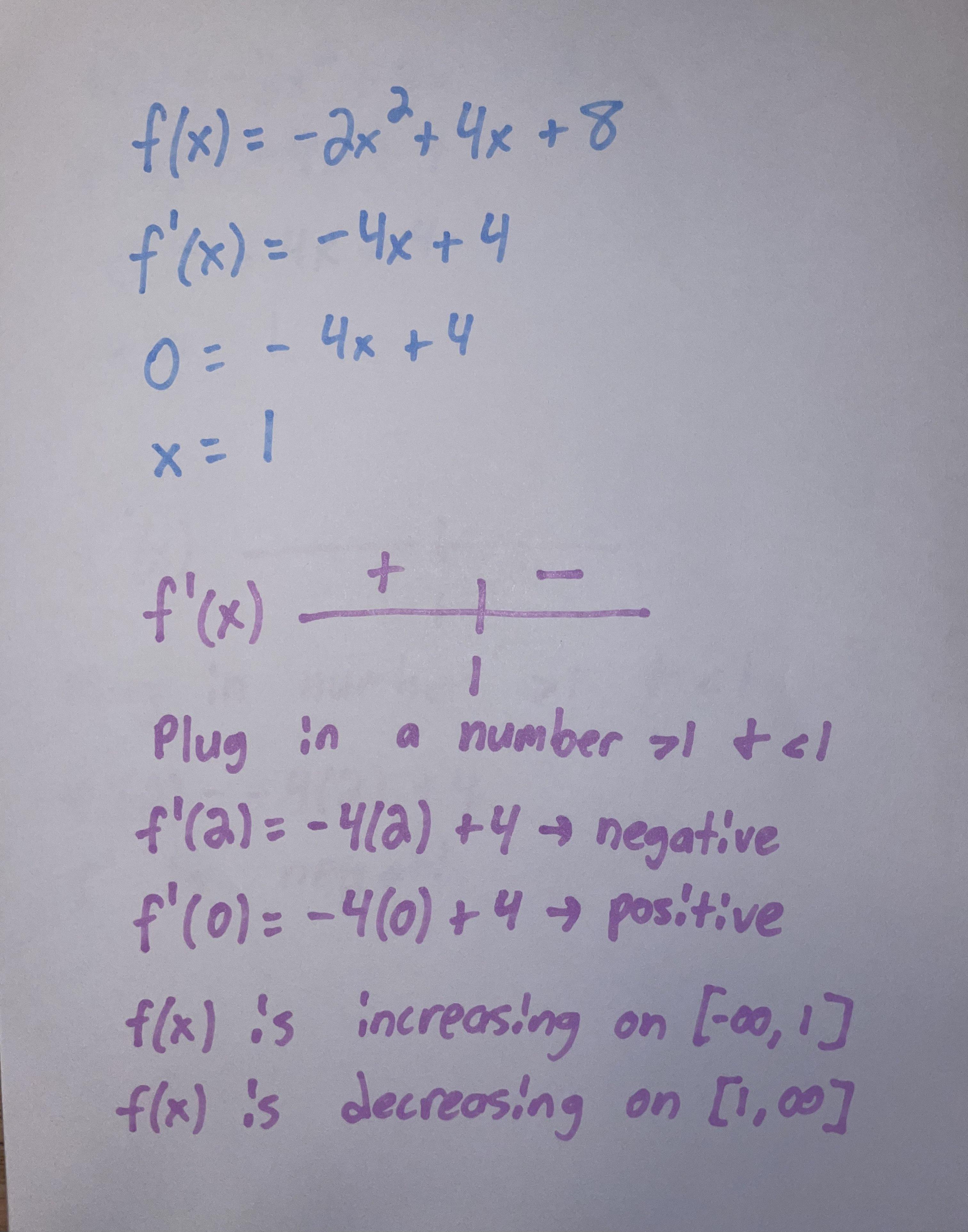
A practical sign-chart workflow (often shown in notes as “pick a test value on each side”) looks like this:

1. Take the derivative of the function.
2. Set f'(x)=0 to find your critical numbers.
3. Pick a test value in each interval determined by the critical numbers and evaluate the sign of f'(x).

The picture below is a typical “test points” setup for checking the sign of f'(x) around a critical number.

Example 1: Using the First Derivative Test

Suppose %%LATEX41%%. Find where %%LATEX42%% increases and decreases and classify critical numbers.

Step 1: Find critical numbers.

Set f'(x)=0:

(x-2)^2(x+1)=0

So critical numbers are %%LATEX45%% and %%LATEX46%%.

Step 2: Make a sign chart for f'(x).

The factor %%LATEX48%% is always nonnegative and is zero only at %%LATEX49%%. It does not change sign across x=2 because the exponent is even.

The sign of %%LATEX51%% is therefore governed by %%LATEX52%% except at x=2 where it becomes zero.

• For %%LATEX54%%, %%LATEX55%%, so f'(x)

Conclusions

• %%LATEX63%% decreases on %%LATEX64%%.
• %%LATEX65%% increases on %%LATEX66%% and (2,\infty).
• At %%LATEX68%%, %%LATEX69%% changes from negative to positive, so %%LATEX70%% has a local minimum at %%LATEX71%%.
• At %%LATEX72%%, %%LATEX73%% does not change sign (positive on both sides), so x=2 is not a local extremum. It is a flat point where the graph keeps increasing.

Worked example: Increase and decrease for a polynomial

Let f(x)=x^3-6x^2+9x+2. Find the intervals where the function is increasing or decreasing.

Differentiate:

f'(x)=3x^2-12x+9

Set f'(x)=0:

3x^2-12x+9=0

Factor:

3(x-1)(x-3)=0

Critical numbers are %%LATEX80%% and %%LATEX81%%.

Now test signs of f'(x)=3(x-1)(x-3) on the intervals:

• If %%LATEX83%%, then %%LATEX84%% and %%LATEX85%%, so %%LATEX86%% and f is increasing.
• If %%LATEX88%%, then %%LATEX89%% and %%LATEX90%%, so %%LATEX91%% and f is decreasing.
• If %%LATEX93%%, then %%LATEX94%% and %%LATEX95%%, so %%LATEX96%% and f is increasing.

Therefore, %%LATEX98%% is increasing on %%LATEX99%% and %%LATEX100%% and decreasing on %%LATEX101%%.

Relative extrema (local extrema)

The first derivative sign changes also tell you relative extrema:

• If %%LATEX102%% shifts from positive to negative at %%LATEX103%%, then %%LATEX104%% has a relative maximum at %%LATEX105%%.
• If %%LATEX106%% shifts from negative to positive at %%LATEX107%%, then %%LATEX108%% has a relative minimum at %%LATEX109%%.

Using the polynomial example above, %%LATEX110%% changes from positive to negative at %%LATEX111%%, so %%LATEX112%% has a relative maximum at %%LATEX113%%. Also, %%LATEX114%% changes from negative to positive at %%LATEX115%%, so %%LATEX116%% has a relative minimum at %%LATEX117%%.

Connecting %%LATEX118%% and %%LATEX119%% graphs

AP questions often give you the graph of %%LATEX120%% (or a sign chart) and ask you about %%LATEX121%%. The translation is systematic:

• Where %%LATEX122%% is above the %%LATEX123%%-axis, f is increasing.
• Where %%LATEX125%% is below the %%LATEX126%%-axis, f is decreasing.
• Zeros of %%LATEX128%% indicate critical numbers of %%LATEX129%%.
• A sign change in %%LATEX130%% at a zero indicates a local extremum of %%LATEX131%%.

A frequent pitfall: if %%LATEX132%% but the graph of %%LATEX133%% just touches the axis and turns around (no sign change), then %%LATEX134%% has no local extremum at %%LATEX135%%.

Exam Focus

• Typical question patterns
  • Given %%LATEX136%% (formula, table, or graph), identify intervals of increase and decrease and local extrema of %%LATEX137%%.
  • Find critical numbers and classify them using a sign chart.
  • Interpret a verbal description (“increasing then decreasing”) in derivative language.
• Common mistakes
  • Declaring “local max or min” whenever f'(c)=0 without checking the sign change.
  • Forgetting that %%LATEX139%% undefined can also create a critical number (if %%LATEX140%% is in the domain).
  • Mixing up increasing and decreasing by reading a derivative graph as if it were the original function.

Absolute Extrema on Closed Intervals (and why endpoints matter)

Local (relative) extrema describe what happens near a point; absolute extrema describe the highest or lowest function value on an entire interval. In applications, absolute extrema are usually what you care about: the maximum profit, minimum cost, greatest distance, smallest surface area, and so on.

The maximum and minimum values are called extrema, and each comes in two types:

• Absolute (global): no other function value on the interval is higher or lower.
• Local (relative): the highest or lowest only in a nearby neighborhood.

The Extreme Value Theorem (EVT)

The Extreme Value Theorem says:

If %%LATEX141%% is continuous on a closed interval %%LATEX142%%, then %%LATEX143%% attains both an absolute maximum value and an absolute minimum value somewhere on %%LATEX144%%.

This theorem matters because it guarantees that absolute extrema actually exist under the right conditions.

• The interval must be closed (endpoints included).
• The interval must be bounded (finite length).
• The function must be continuous on the interval.

A classic counterexample: %%LATEX145%% on %%LATEX146%% is continuous on that interval, but there is no absolute maximum because values blow up near 0, which is not included.

How to find absolute maxima and minima (Candidate’s Test)

On a closed interval %%LATEX148%% where %%LATEX149%% is continuous, the procedure is reliable. This is often called the Candidate’s Test:

1. Find critical numbers of %%LATEX150%% in %%LATEX151%%.
2. Evaluate f at each critical number.
3. Evaluate %%LATEX153%% and %%LATEX154%%.
4. Compare all those function values. The largest is the absolute maximum value; the smallest is the absolute minimum value.

A common presentation is to make a table of candidate %%LATEX155%%-values (endpoints plus critical numbers) and plug those into the original function (not into %%LATEX156%%).

Why endpoints are included: absolute extrema can occur at the edges. Even though endpoints are not critical numbers (derivatives describe interior behavior), they are still candidates for absolute extrema on a closed interval.

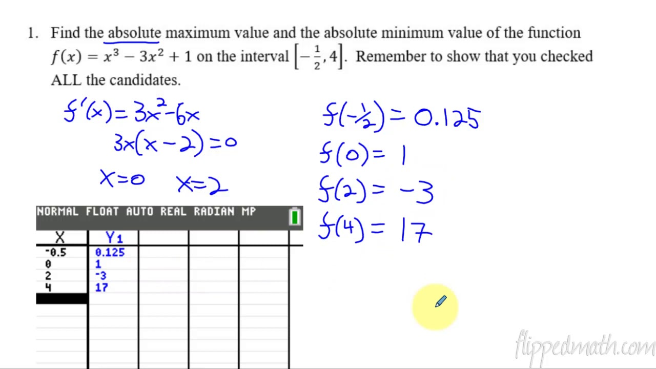
Example 2: Absolute extrema on an interval

Find the absolute maximum and minimum of %%LATEX157%% on %%LATEX158%%.

Step 1: Differentiate and find critical numbers in the interior.

f'(x)=3x^2-6x

Set f'(x)=0:

3x^2-6x=0

3x(x-2)=0

Critical numbers: %%LATEX163%% and %%LATEX164%%. Only %%LATEX165%% is in the interior %%LATEX166%%. (The value x=0 is an endpoint here.)

Step 2: Evaluate f at interior critical numbers and endpoints.

f(0)=1

f(2)=8-12+1=-3

f(3)=27-27+1=1

Step 3: Compare values.

The smallest value is %%LATEX172%% at %%LATEX173%%, so the absolute minimum is f(2)=-3.

The largest value is %%LATEX175%%, which occurs at both %%LATEX176%% and %%LATEX177%%, so the absolute maximum value is %%LATEX178%% at %%LATEX179%% and %%LATEX180%%.

When the method fails (and what that tells you)

If the function is not continuous on [a,b], EVT does not apply, and absolute extrema might not exist. Even if extrema exist, the “check endpoints and critical points” recipe can miss behavior near discontinuities or vertical asymptotes.

Also, if the interval is open (like (a,b) ), a function can approach a supremum or infimum without attaining it.

Exam Focus

• Typical question patterns
  • “Find the absolute maximum or minimum of %%LATEX183%% on %%LATEX184%% and justify your answer.”
  • Identify whether EVT guarantees extrema for a given function and interval.
  • Compare values at critical points and endpoints using exact values (not decimal guesses).
• Common mistakes
  • Forgetting to check endpoints when asked for absolute extrema.
  • Finding critical numbers but evaluating %%LATEX185%% instead of %%LATEX186%% when comparing candidates.
  • Applying EVT even when the function is discontinuous (for example, rational functions with vertical asymptotes inside the interval).

Mean Value Theorem and Rolle’s Theorem (turning average change into instant change)

Derivatives are instantaneous rates, but many real situations start with an average rate: average speed over a trip, average growth over a year, average temperature change over a day. The big idea of the Mean Value Theorem (MVT) is that under the right smoothness conditions, an instantaneous rate must equal that average rate at some point.

Secant slopes vs tangent slopes

Given two points %%LATEX187%% and %%LATEX188%%, the slope of the secant line is the average rate of change:

\frac{f(b)-f(a)}{b-a}

A tangent line slope at %%LATEX190%% is %%LATEX191%%.

MVT connects these two slopes. Many students summarize it as: “somewhere between the endpoints, a tangent line has the same slope as the secant line.”

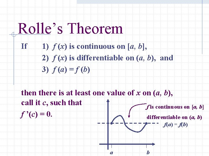
Rolle’s Theorem

Rolle’s Theorem is a special case of MVT. If:

• %%LATEX192%% is continuous on %%LATEX193%%,
• %%LATEX194%% is differentiable on %%LATEX195%%,
• f(a)=f(b),

then there exists at least one %%LATEX197%% in %%LATEX198%% such that:

f'(c)=0

Intuition: if you start and end at the same height on a smooth curve, you must have had at least one horizontal tangent somewhere in between.

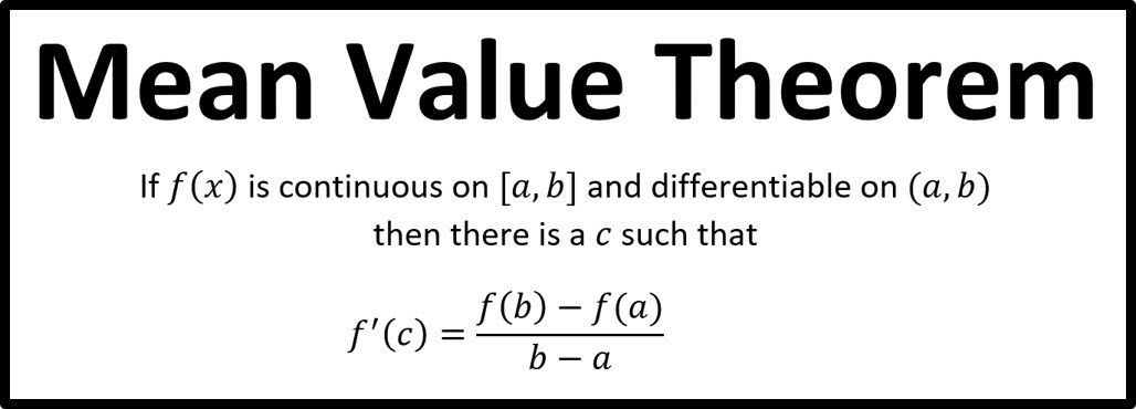
The Mean Value Theorem (MVT)

If:

• %%LATEX200%% is continuous on %%LATEX201%%,
• %%LATEX202%% is differentiable on %%LATEX203%%,

then there exists at least one %%LATEX204%% in %%LATEX205%% such that:

f'(c)=\frac{f(b)-f(a)}{b-a}

This theorem is foundational because it justifies many “there exists a point where…” conclusions.

A common error is to use MVT without checking conditions. On AP free response, you are often expected to explicitly state continuity and differentiability, especially for piecewise functions.

Example 3: Finding a value guaranteed by MVT

Let %%LATEX207%% on %%LATEX208%%.

Step 1: Check conditions.

%%LATEX209%% is a polynomial, so it is continuous on %%LATEX210%% and differentiable on (1,3) .

Step 2: Compute the average rate of change.

\frac{f(3)-f(1)}{3-1}=\frac{9-1}{2}=4

Step 3: Find %%LATEX213%% such that %%LATEX214%%.

f'(x)=2x

Set %%LATEX216%%, so %%LATEX217%%.

So MVT guarantees at least one point c=2 where the instantaneous slope equals the average slope.

Interpreting MVT in real contexts

If s(t) is position, then:

\frac{s(b)-s(a)}{b-a}

is average velocity on [a,b], and MVT says there is a time when the instantaneous velocity equals that average velocity.

This is the calculus justification for statements like “At some point during the trip, your speedometer read exactly your average speed.”

Consequences you should understand

• If %%LATEX222%% for all %%LATEX223%% in an interval, then f is constant on that interval.
• If %%LATEX225%% for all %%LATEX226%% in an interval, then %%LATEX227%% is increasing on that interval (and similarly for %%LATEX228%%).

These facts are often proven using MVT, and AP questions sometimes ask you to use MVT logic to justify monotonicity.

Exam Focus

• Typical question patterns
  • Verify MVT conditions for a given function (often piecewise) and then find a value of c.
  • Interpret MVT in context (average velocity implies a time with that instantaneous velocity).
  • Use Rolle’s Theorem to argue existence of a point where f'(c)=0.
• Common mistakes
  • Forgetting to state and check continuity on %%LATEX231%% and differentiability on %%LATEX232%%.
  • Solving %%LATEX233%% but giving a %%LATEX234%% outside (a,b) .
  • Confusing secant slope with tangent slope and mixing up which one is average vs instantaneous.

Concavity and the Second Derivative (how the graph “bends”)

The first derivative tells you whether a function is increasing or decreasing. The second derivative tells you how that increase or decrease is changing, meaning whether the function’s slope is getting larger or smaller. Geometrically, this is the idea of concavity.

What concavity means

A function is concave up on an interval if its graph bends like a cup: as you move left to right, tangent slopes increase (they become more positive, or less negative). A function is concave down if it bends like a cap: tangent slopes decrease.

The second derivative captures this:

• If %%LATEX236%% on an interval, %%LATEX237%% is concave up there.
• If %%LATEX238%% on an interval, %%LATEX239%% is concave down there.

Another helpful phrasing is “increasing, but at a decreasing rate” (or “decreasing, but at an increasing rate”). This is exactly what concavity describes.

A common visual summary is shown here.

Inflection points

An inflection point is a point on the graph where concavity changes (concave up to concave down, or vice versa). A necessary step to find candidates is to locate where %%LATEX240%% or where %%LATEX241%% is undefined, but a candidate is only an actual inflection point if the concavity truly changes sign.

A common mistake is to say “%%LATEX242%% implies an inflection point.” That is not guaranteed. You must check for a sign change in %%LATEX243%%.

A sign-chart workflow for concavity often looks like this:

1. Take the second derivative.
2. Set %%LATEX244%% to find candidate inflection %%LATEX245%%-values.
3. Verify a sign change in f''(x) by testing points in the intervals.

The Second Derivative Test (classifying local extrema)

If %%LATEX247%% is a critical number with %%LATEX248%% and f''(c) exists, then:

• If %%LATEX250%%, %%LATEX251%% has a local minimum at c.
• If %%LATEX253%%, %%LATEX254%% has a local maximum at c.
• If f''(c)=0, the test is inconclusive.

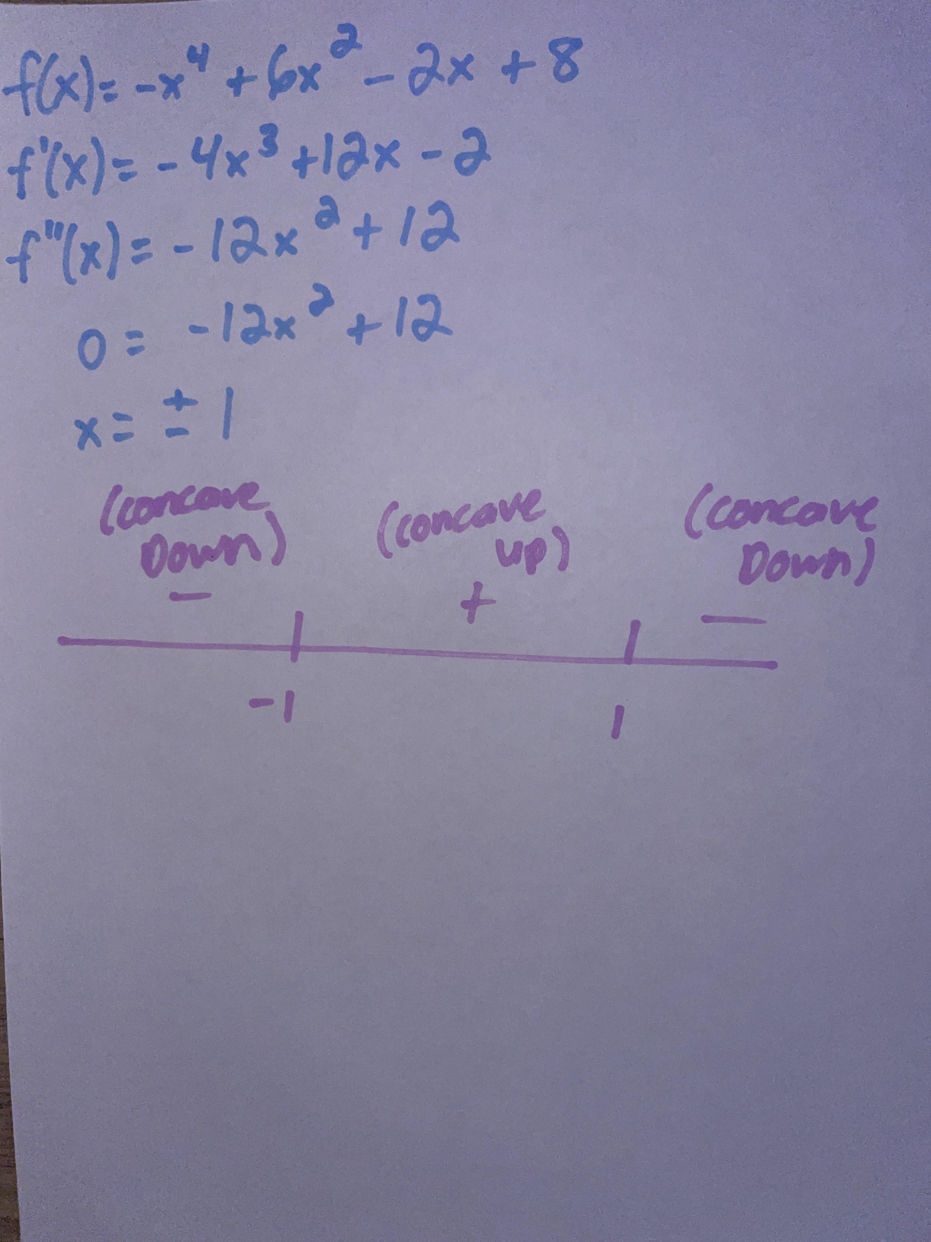
Example 4: Concavity, inflection, and classification

Let f(x)=x^4-4x^3.

Step 1: Compute derivatives.

f'(x)=4x^3-12x^2=4x^2(x-3)

f''(x)=12x^2-24x=12x(x-2)

Step 2: Concavity from f''.

Candidates come from f''(x)=0:

12x(x-2)=0

So %%LATEX263%% and %%LATEX264%% are candidates.

Check signs of f'':

• For %%LATEX266%%, %%LATEX267%%, thus %%LATEX268%% and %%LATEX269%% is concave up.
• For %%LATEX270%%, %%LATEX271%%, thus %%LATEX272%% and %%LATEX273%% is concave down.
• For %%LATEX274%%, %%LATEX275%%, thus %%LATEX276%% and %%LATEX277%% is concave up.

Concavity changes at both %%LATEX278%% and %%LATEX279%%, so both correspond to inflection points.

Step 3: Local extrema from f'.

Set f'(x)=0:

4x^2(x-3)=0

Critical numbers: %%LATEX283%% and %%LATEX284%%.

• For %%LATEX285%%, %%LATEX286%% and %%LATEX287%%, so there is a local minimum at %%LATEX288%%.
• For %%LATEX289%%, %%LATEX290%% but %%LATEX291%%, so the second derivative test is inconclusive. In fact, because of the %%LATEX292%% factor, %%LATEX293%% does not change sign at %%LATEX294%%, so x=0 is not a local extremum.

Worked example: Concavity for a polynomial

Suppose %%LATEX296%%. Find intervals where %%LATEX297%% is concave up or concave down.

Differentiate twice:

f'(x)=3x^2-12x+9

f''(x)=6x-12

Set f''(x)=0:

6x-12=0

x=2

Test intervals:

• If %%LATEX303%%, then %%LATEX304%%, so %%LATEX305%% is concave down on %%LATEX306%%.
• If %%LATEX307%%, then %%LATEX308%%, so %%LATEX309%% is concave up on %%LATEX310%%.

Exam Focus

• Typical question patterns
  • Find intervals of concavity and identify inflection points using f'' sign changes.
  • Use the second derivative test to classify a critical point (when applicable).
  • Given a graph of %%LATEX312%%, infer concavity of %%LATEX313%% (concave up where f' increases).
• Common mistakes
  • Claiming “inflection point at f''=0” without checking a concavity change.
  • Confusing concavity with increasing and decreasing (they are controlled by different derivatives).
  • Applying the second derivative test when %%LATEX316%% is not zero or when %%LATEX317%% does not exist.

Building a Complete Function Analysis (sign charts and curve sketching logic)

Many AP problems ask you to analyze a function: find critical points, intervals of increase and decrease, concavity, inflection points, and sometimes sketch a reasonable graph. The point is not artistic drawing; it is demonstrating that you understand how derivative information constrains the behavior of f.

A structured way to organize analysis

When you have a formula for f:

1. Domain: determine where f is defined.
2. First derivative: compute f'(x).
3. Critical numbers: solve %%LATEX322%% and check where %%LATEX323%% is undefined (but f is defined).
4. Increasing/decreasing: use a sign chart for f'(x).
5. Second derivative: compute f''(x).
6. Concavity/inflection: use a sign chart for f''(x).
7. Extrema: classify with the first derivative test (or second derivative test when appropriate).

This workflow prevents a common issue: trying to “spot” behavior from algebra without systematically checking signs.

When you are given graphs or tables instead of formulas

AP frequently gives you the graph of %%LATEX328%% or a table of values and asks about %%LATEX329%%. In those situations, you do not differentiate; you interpret.

Reliable translations:

• %%LATEX330%% is increasing where %%LATEX331%%.
• %%LATEX332%% is decreasing where %%LATEX333%%.
• %%LATEX334%% has a local maximum where %%LATEX335%% changes from positive to negative.
• %%LATEX336%% has a local minimum where %%LATEX337%% changes from negative to positive.
• %%LATEX338%% is concave up where %%LATEX339%% is increasing.
• %%LATEX340%% is concave down where %%LATEX341%% is decreasing.

And in terms of f'':

• %%LATEX343%% means %%LATEX344%% is increasing.
• %%LATEX345%% means %%LATEX346%% is decreasing.

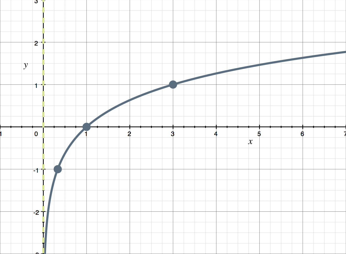
Example 5: Full analysis from a formula

Analyze %%LATEX347%% on the domain %%LATEX348%%.

Step 1: Derivative and critical numbers.

f'(x)=1-\frac{1}{x^2}

Solve f'(x)=0:

1-\frac{1}{x^2}=0

\frac{1}{x^2}=1

x^2=1

Given %%LATEX354%%, the only critical number is %%LATEX355%%.

Step 2: Increasing/decreasing via sign of f'.

For %%LATEX357%%, %%LATEX358%%, so %%LATEX359%% and %%LATEX360%% is decreasing.

For %%LATEX361%%, %%LATEX362%%, so %%LATEX363%% and %%LATEX364%% is increasing.

So %%LATEX365%% decreases then increases, meaning %%LATEX366%% is a local minimum.

Step 3: Concavity.

f''(x)=\frac{2}{x^3}

For %%LATEX368%%, %%LATEX369%%, so f is concave up everywhere on its domain and has no inflection points.

A note on reasoning and justification

On free-response questions, it often is not enough to list an answer. You may need to explicitly connect your conclusion to derivative sign changes.

Good justification sounds like: “Since %%LATEX371%% changes from positive to negative at %%LATEX372%%, %%LATEX373%% changes from increasing to decreasing, so %%LATEX374%% has a local maximum at x=c.”

Exam Focus

• Typical question patterns
  • Complete a table of intervals (increasing/decreasing, concave up/down) and mark local extrema and inflection points.
  • Given %%LATEX376%% as a graph, identify where %%LATEX377%% has extrema and where f is concave up/down.
  • Provide written justification using sign analysis.
• Common mistakes
  • Treating “critical numbers of %%LATEX379%%” (where %%LATEX380%%) as if they were automatically extrema of f.
  • Marking inflection points without verifying a concavity sign change.
  • Forgetting domain restrictions (for example, analyzing behavior at x=0 when the function is not defined there).

Optimization (modeling a real problem into a calculus problem)

Optimization is the process of finding the maximum or minimum value of a quantity under given constraints. The calculus insight is that optimal values typically occur where the derivative is zero (flat tangent) or at boundary points.

Optimization is not just “take a derivative and set it to zero.” The hardest part is often modeling: choosing variables, building an objective function, and correctly handling constraints and domains.

The standard optimization strategy

1. Define variables clearly.
2. Write the objective function (what you maximize or minimize).
3. Use constraints to reduce to one variable.
4. Determine the feasible domain (often a closed interval).
5. Differentiate and find critical numbers in the interior.
6. Check endpoints and critical numbers (absolute extrema method) and interpret.

A crucial conceptual point: your final answer should be in the units and quantities of the original problem, not just “x=3.” Often you must compute additional dimensions.

Why endpoints matter in optimization

Many physical constraints create a closed interval: lengths cannot be negative, dimensions may be capped by available material, etc. Even if the derivative never equals zero, the optimum might occur at the boundary.

Example 6: Classic fencing optimization

You have 200 meters of fencing to enclose a rectangular area. What dimensions maximize the area?

Step 1: Define variables.

Let %%LATEX384%% be the length and %%LATEX385%% be the width in meters.

Step 2: Constraint equation (perimeter).

2x+2y=200

So:

y=100-x

Step 3: Objective function (area).

A=xy

Substitute the constraint:

A(x)=x(100-x)=100x-x^2

Step 4: Domain.

You need %%LATEX390%% and %%LATEX391%%. Since %%LATEX392%%, that means %%LATEX393%%.

Step 5: Differentiate and find critical points.

A'(x)=100-2x

Set A'(x)=0:

100-2x=0

x=50

Then y=100-50=50.

Step 6: Interpret.

The area is maximized when the rectangle is a square: %%LATEX399%% m by %%LATEX400%% m.

Example 7: Minimizing distance to a point on a line

Find the point on the line %%LATEX401%% closest to the point %%LATEX402%%.

Step 1: Variable point and distance.

Let the point on the %%LATEX403%%-axis be %%LATEX404%%.

Distance:

D=\sqrt{(x-2)^2+(0-3)^2}=\sqrt{(x-2)^2+9}

Step 2: Simplify objective (avoid the square root).

Because the square root is increasing, minimizing D is equivalent to minimizing:

D^2=(x-2)^2+9

Step 3: Differentiate.

\frac{d}{dx}D^2=2(x-2)

Set to zero:

2(x-2)=0

x=2

So the closest point is Q(2,0).

Common modeling pitfalls

• Not defining the domain, leading to impossible “optimal” values.
• Treating multiple variables as independent when constraints link them.
• Forgetting what the question asked for (for example, returning x when it asked for dimensions or maximum area value).

Exam Focus

• Typical question patterns
  • Set up an objective function from a word problem and use derivatives to find the max or min.
  • Optimization with geometry (rectangles, boxes, distance problems).
  • “Justify that your critical point gives a minimum or maximum” using first derivative sign change or second derivative.
• Common mistakes
  • Skipping the constraint step and differentiating an objective that still has two variables.
  • Ignoring endpoints even when the feasible set is a closed interval.
  • Giving a critical number but not translating it back into the quantities requested (dimensions, time, cost, etc.).

Motion Along a Line (position, velocity, acceleration, and speed)

Motion problems are one of the most natural applications of derivatives.

The core quantities and their meanings

Let %%LATEX413%% be the position of an object along a line at time %%LATEX414%%.

Velocity is the derivative of position:

v(t)=s'(t)

Acceleration is the derivative of velocity (and the second derivative of position):

a(t)=v'(t)=s''(t)

Speed is the magnitude of velocity:

|v(t)|

Moving right/left and turning around

• If v(t)>0, the object moves to the right.
• If v(t)

A direction change occurs when velocity changes sign, which often happens at a time when v(t)=0 (but you still check the sign change).

Speeding up vs slowing down

• The object is speeding up when speed is increasing.
• The object is slowing down when speed is decreasing.

Key rule:

• Speed increases when velocity and acceleration have the same sign.
• Speed decreases when velocity and acceleration have opposite signs.

Displacement vs distance traveled

Over a time interval [a,b]:

Displacement is net change in position:

s(b)-s(a)

Distance traveled is the integral of speed:

\int_a^b |v(t)|dt

In practice on AP, distance traveled is often computed by splitting the interval at times when v(t)=0 and summing absolute displacements.

Example 8: Interpreting motion from formulas

Let:

s(t)=t^3-6t^2+9t

for 0\le t\le 5.

Step 1: Velocity and acceleration.

v(t)=s'(t)=3t^2-12t+9

a(t)=v'(t)=6t-12

Step 2: When is the particle at rest?

Set v(t)=0:

3t^2-12t+9=0

Divide by 3:

t^2-4t+3=0

Factor:

(t-1)(t-3)=0

So the particle is at rest at %%LATEX435%% and %%LATEX436%%.

Step 3: Direction via sign of v(t).

Because v(t)=3(t-1)(t-3):

• For %%LATEX439%%, %%LATEX440%%, moving right.
• For %%LATEX441%%, %%LATEX442%%, moving left.
• For %%LATEX443%%, %%LATEX444%%, moving right.

Step 4: Speeding up and slowing down.

Acceleration is a(t)=6(t-2).

• For %%LATEX446%%, %%LATEX447%%.
• For %%LATEX448%%, %%LATEX449%%.

Compare signs of %%LATEX450%% and %%LATEX451%%:

• On %%LATEX452%%: %%LATEX453%% and a

Exam Focus

• Typical question patterns
  • Given %%LATEX464%% or %%LATEX465%%, find when the particle changes direction, is at rest, speeds up, or slows down.
  • Compute displacement and distance traveled over an interval (often using sign changes of v).
  • Interpret the meaning of positive and negative velocity and acceleration in context.
• Common mistakes
  • Confusing velocity with speed (forgetting the absolute value for speed).
  • Saying “speeding up when %%LATEX467%%” without considering the sign of %%LATEX468%%.
  • Computing distance traveled as s(b)-s(a) even when there is a direction change.

Using Derivative Information Presented in Tables, Graphs, or Verbal Descriptions

Not every AP question gives you a nice formula. A major skill in analytical applications is translating between multiple representations: function values, derivative values, graphs, and real-world statements.

Reading behavior from a table of derivative values

If you are given a table with values of %%LATEX470%% at certain points, you can sometimes infer increasing or decreasing on intervals between those points, but only if the problem also gives you a reason to assume the sign does not change between sample points (for example, if %%LATEX471%% is continuous and only crosses zero at listed points). Otherwise, isolated table values alone do not guarantee what happens in between.

AP problems often avoid ambiguity by providing:

• a graph (continuous picture), or
• a statement like “%%LATEX472%% is continuous” plus zeros of %%LATEX473%%, or
• monotonic behavior of f'.

The high-level skill is: do not overclaim. If the data does not guarantee a sign, you must say you cannot conclude.

Reading behavior from the graph of f

When you are given the graph of f itself:

• Increasing and decreasing: look at whether the graph goes up or down left-to-right.
• Local maxima and minima: look for peaks and valleys (and note corners can create extrema).
• Concavity: look at whether slopes are increasing (concave up) or decreasing (concave down).

Then connect these to derivative statements:

• At a smooth local extremum, f'(c)=0.
• At a corner or cusp, f'(c) may not exist.
• At an inflection point, f'' changes sign.

Reading behavior from the graph of f'

Treat %%LATEX481%% like the control panel for %%LATEX482%%.

• Zeros of %%LATEX483%% are where %%LATEX484%% has horizontal tangents or nondifferentiable points (if described).
• Regions where f' is positive or negative give increasing or decreasing.
• Where %%LATEX486%% increases or decreases gives concavity of %%LATEX487%%.

Example 9: Translating a verbal description into calculus statements

Suppose you are told:

• %%LATEX488%% is differentiable on %%LATEX489%%.
• %%LATEX490%% is increasing on %%LATEX491%%.
• %%LATEX492%% is decreasing on %%LATEX493%%.
• %%LATEX494%% is concave down on %%LATEX495%%.
• %%LATEX496%% is concave up on %%LATEX497%%.

From this you can conclude:

• Since %%LATEX498%% changes from increasing to decreasing at %%LATEX499%%, %%LATEX500%% has a local maximum at %%LATEX501%%.
• Since concavity changes at %%LATEX502%%, %%LATEX503%% has an inflection point at x=2.
• Because %%LATEX505%% is concave down on %%LATEX506%%, %%LATEX507%% is decreasing there; because %%LATEX508%% is concave up on %%LATEX509%%, %%LATEX510%% is increasing there.

Exam Focus

• Typical question patterns
  • Given a graph of %%LATEX511%%, determine where %%LATEX512%% is increasing or decreasing and where f is concave up or down.
  • Use sign changes of %%LATEX514%% to identify local maxima and minima of %%LATEX515%%.
  • Determine what can and cannot be concluded from a table of values.
• Common mistakes
  • Overinterpreting sparse table data as if it guarantees sign behavior between points.
  • Confusing “%%LATEX516%% is increasing” with “%%LATEX517%% is increasing”.
  • Assuming differentiability at a point just because the graph looks smooth at a quick glance (corners and cusps matter).