AP Environmental Science: Population Dynamics and Biological Strategies
Generalist and Specialist Species
In ecology, the way a species interacts with its environment—specifically its niche (role)—determines its ability to survive environmental changes. This classification typically falls into two categories: Generalists and Specialists.
Generalist Species
A generalist species is capable of surviving in a wide variety of environmental conditions and can make use of a range of different resources.
- Broad Niche: They can live in many places, eat a variety of foods, and tolerate a wide range of environmental conditions.
- Adaptability: High. They are likely to become invasive species when introduced to non-native habitats because they can easily adapt.
- Examples: Raccoons (eat almost anything, live in cities or forests), Rats, Cockroaches, Humans.
Specialist Species
A specialist species can thrive only in a narrow range of environmental conditions or has a limited diet.
- Narrow Niche: They may require a specific habitat, specific food source, or narrow temperature range.
- Adaptability: Low. They are more prone to extinction when environmental conditions change (e.g., habitat loss).
- Examples: Giant Pandas (eat almost exclusively bamboo), Koalas (eucalyptus), Salamanders (require specific moisture levels).
Comparison Summary:
| Feature | Generalist | Specialist |
|---|---|---|
| Niche Width | Broad | Narrow |
| Diet | Varied | Specific |
| Habitat Tolerance | High | Low |
| Response to Change | Resilient | Fragile |
| Competition Advantage | Outcompetes in changing environments | Outcompetes in constant/stable environments |
Reproductive Strategies: K-Selected and r-Selected Species
Species organize their energy into reproduction and survival differently. This trade-off is often described using the variables $r$ (growth rate) and $K$ (carrying capacity) from population growth equations.
K-Selected Species
These species effectively compete for resources and usually exist near the Carrying Capacity ($K$) of their environment.
- Characteristics: Large body size, long life span, late reproductive maturity.
- Reproduction: Few offspring, but high investment in parental care.
- Stability: Thrive in stable environments where competition is high.
- Examples: Elephants, Whales, Humans, Saguaro Cactus.
r-Selected Species
These species prioritize a high intrinsic growth rate ($r$). They maximize Biotic Potential (the maximum reproductive capacity of an organism under optimum environmental conditions).
- Characteristics: Small body size, short life span, early maturity.
- Reproduction: Many offspring, low or no parental care.
- Stability: Thrive in disturbed or unstable environments; often pioneer species.
- Examples: Bacteria, Insects, Rodents, Dandelions.
The Continuum
It is crucial to remember that $K$ and $r$ selection are ends of a spectrum. Some organisms generally considered $K$-selected (like sea turtles) may produce many eggs (an $r$-trait) but live very long lives (a $K$-trait).
Survivorship Curves
A Survivorship Curve is a graph showing the number or proportion of individuals surviving to each age for a given species or group (cohort). These curves correlate strongly with reproductive strategies.
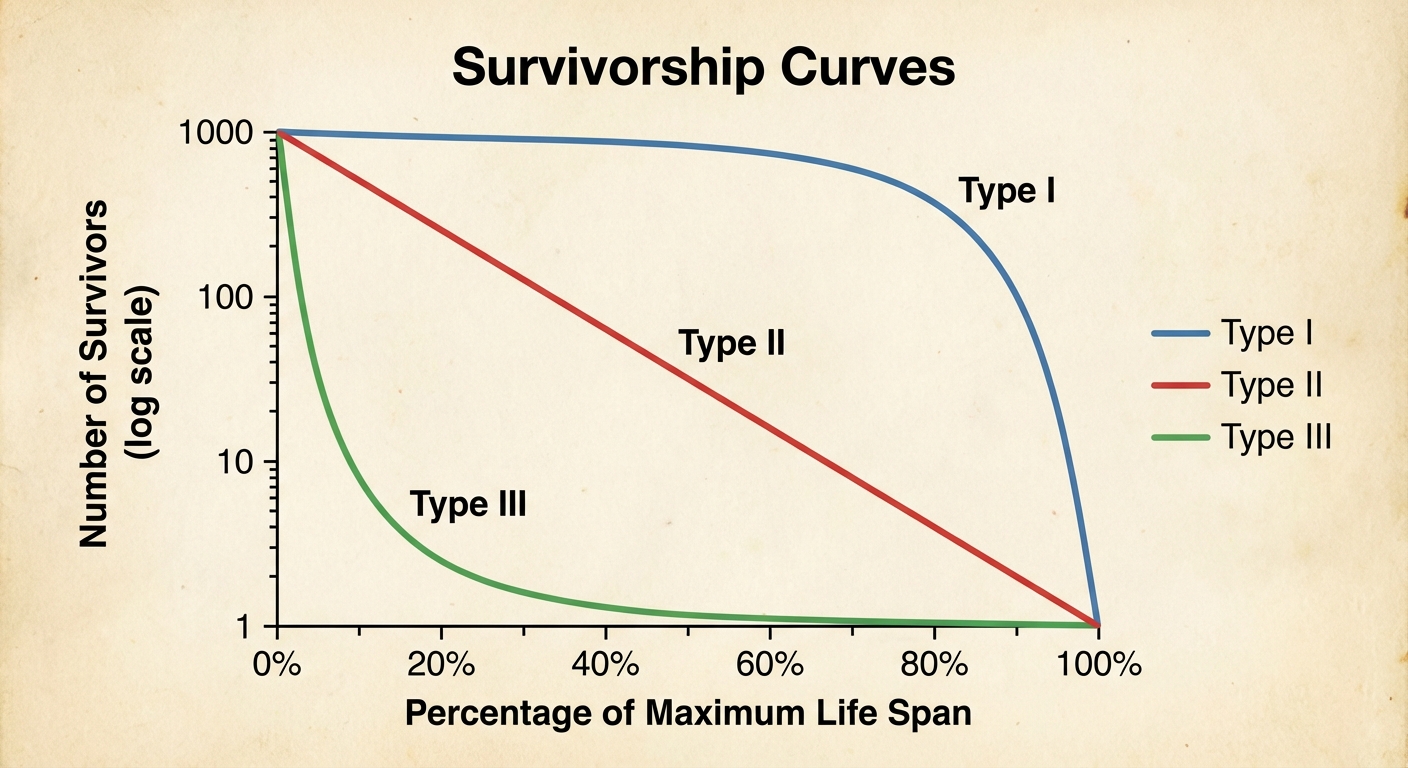
Type I (Late Loss)
- Pattern: High survival throughout most of the life span; mortality increases significantly in old age.
- Key Drivers: High parental care and protection significantly reduce early mortality.
- Correlation: Typical of K-selected species.
- Example: Humans, large mammals.
Type II (Constant Loss)
- Pattern: Roughly constant mortality rate/survival probability is experienced regardless of age.
- Key Drivers: Predation or disease affects all ages equally.
- Correlation: Intermediate species.
- Example: Songbirds, squirrels, coral, some reptiles.
Type III (Early Loss)
- Pattern: Low survivorship early in life; those that do survive the bottleneck live a long time.
- Key Drivers: Producing thousands of offspring with no care relies on sheer numbers to ensure some reach adulthood.
- Correlation: Typical of r-selected species.
- Example: Fish, amphibians, plants (seeds), marine invertebrates.
Carrying Capacity ($K$)
Carrying Capacity ($K$) is defined as the maximum number of individuals in a population that an environment can support significantly over the long term without degrading the resource base.
Limiting Factors
Populations cannot grow indefinitely due to limiting factors. These fall into two categories:
- Density-Dependent Factors: The impact increases as population density increases.
- Examples: Competition for food, spread of disease, predation, and waste accumulation.
- Mechanism: As the population approaches $K$, these factors slow growth.
- Density-Independent Factors: The impact is the same regardless of population size.
- Examples: Natural disasters (hurricanes, floods), fire, droughts, anthropogenic events (pesticide spraying).
Population Growth Models
Understanding how populations change size over time involves two main mathematical models: Exponential Growth and Logistic Growth.
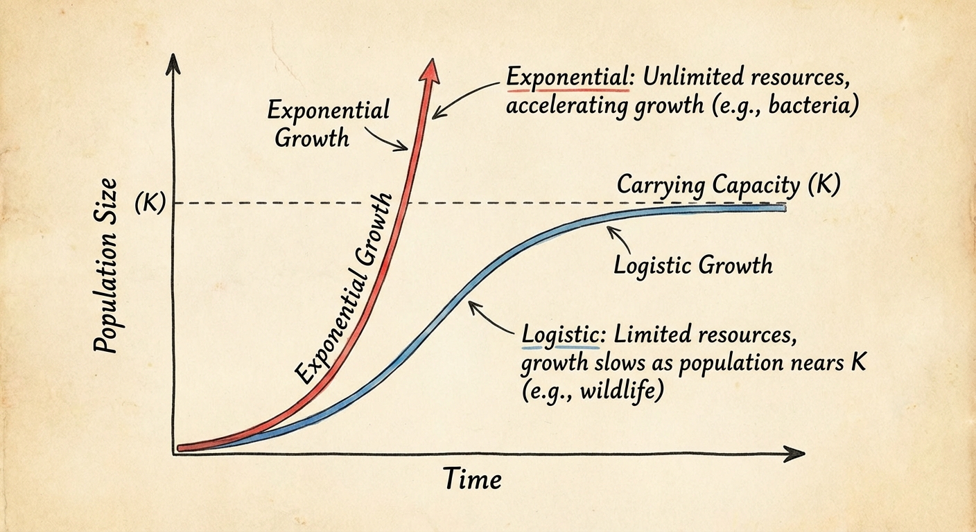
1. Exponential Growth (J-Curve)
Occurs when a population has unlimited resources and no growth restrictions.
- Concepts: The population grows at its intrinsic rate of increase ($r_{max}$).
- Formula:
- Appearance: A graph that starts slow and shoots up vertically (J-shape).
- Context: usually temporary (e.g., invasive species entering a new habitat, bacterial bloom).
2. Logistic Growth (S-Curve)
Occurs when a population's growth slows and stops as it approaches the Carrying Capacity ($K$).
- Concepts: Environmental resistance (limited food, space) pushes back against biotic potential.
- Formula (Conceptual): Growth Rate $\approx rN \left(\frac{K-N}{K}\right)$. Note that as $N$ approaches $K$, growth approaches 0.
- Appearance: S-shaped curve (Sigmoid).
Overshoot and Dieback
In reality, populations rarely experience perfect logistic growth. They often experience Overshoot and Dieback.
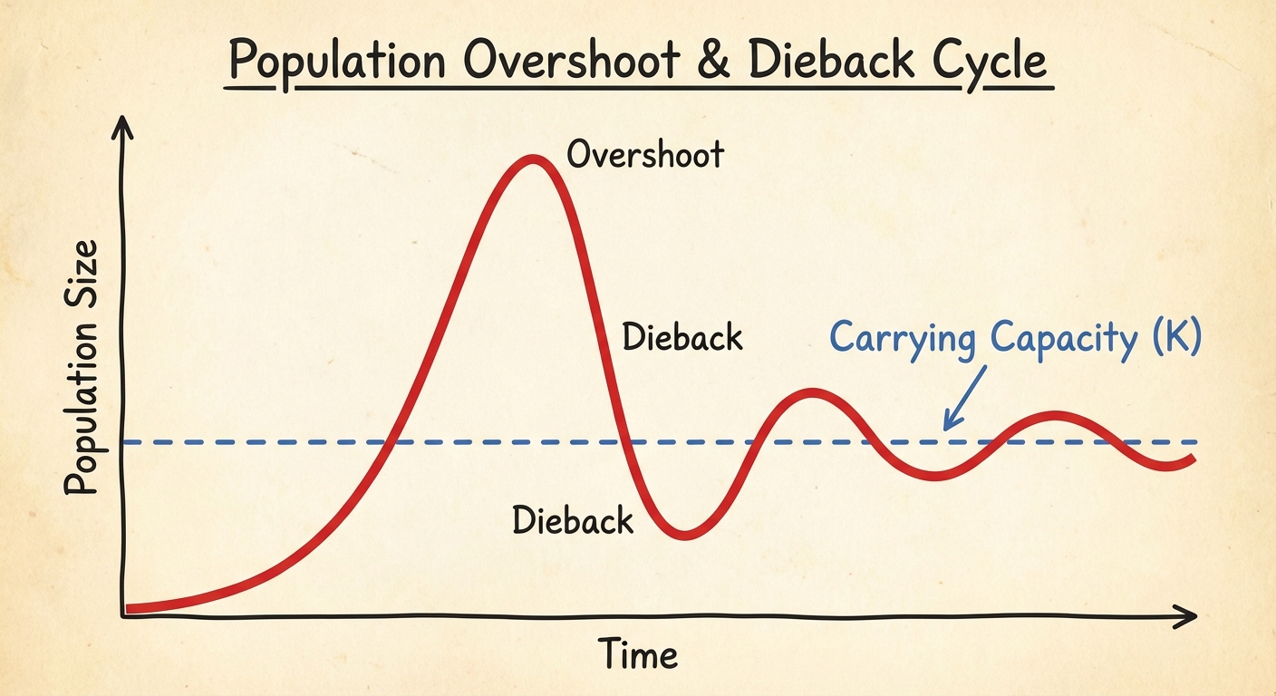
- Overshoot: The population exceeds the carrying capacity because there is a reproductive time lag (species reproduce before resources run out).
- Dieback: Because the environment cannot support the excess numbers (resource depletion), a massive die-off occurs, dropping the population below $K$.
- Consequence: Severe overshoot can degrade the habitat, permanently lowering the carrying capacity ($K$) for the future.
Math Spotlight: The Rule of 70
A quick way to estimate how many years it takes for a population to double at a constant growth rate.
Example: If a population grows at $2\%$, it will double in $70/2 = 35$ years.
Common Mistakes & Pitfalls
- Confusing Rate with Capacity: Students often confuse $r$ (how fast it grows) with $K$ (how many can fit). Remember: $r$ is about speed/reproduction, $K$ is about the environment's limit.
- K-selected $\neq$ Type I always: While highly correlated, do not assume every K-selected species is a perfect Type I curve or vice-versa. Always look at the data provided in the exam question.
- "Survival of the Fittest" Misconception: In the context of Generalists/Specialists, "fittest" depends on the environment. In a stable rainforest, the Specialist is "fitter." In a rapidly urbanizing area, the Generalist is "fitter."
- Growth Rate vs. Population Size: A population can have a decreasing growth rate (e.g., dropping from 3% to 2%) but the total population size is still increasing (just more slowly).
- Density Independence: Students often label starvation as density-independent. It is usually density-dependent because food scarcity creates competition only when the population is large relative to the resource.