AP Calculus AB Unit 1 (Limits & Continuity): Continuity, Discontinuities, IVT, and How to “Fix” Holes
AP Calculus AB Unit 1 (Limits & Continuity): Continuity, Discontinuities, IVT, and How to “Fix” Holes
Defining Continuity at a Point
In everyday geometry, people describe a continuous curve as one you can draw without lifting your pencil. That picture is helpful, but AP Calculus requires a precise, limit-based definition so you can prove continuity from formulas, tables, and graphs.
A function is continuous at a point (at x = c) only when three conditions hold simultaneously. Many teachers call this the Definition of Continuity Checklist:
1) The function value exists: the value is defined.
2) The limit exists: the two-sided limit exists as a finite real number. Equivalently, the one-sided limits both exist and are equal:
3) Limit equals value: the function matches its own limit:
If any condition fails, then the function is discontinuous at that point.

The limit condition uses two-sided limits (built from one-sided limits)
To claim exists, you must check that the left-hand and right-hand limits match. A common trap (especially from graphs) is to read only one side and assume the two-sided limit exists.
A useful notation table
| Idea | Notation | Meaning |
|---|---|---|
| Left-hand limit | approach c from values less than c | |
| Right-hand limit | approach c from values greater than c | |
| Two-sided limit | exists only if left and right limits agree | |
| Continuous at a point | “f is continuous at c” | limit exists and equals |
How to check continuity at a point (a reliable process)
When asked whether a function is continuous at x = c, don’t guess from how smooth the graph looks. Use a consistent reasoning process:
1) Check the function value: compute or read %%LATEX8%%. If %%LATEX9%% is undefined, continuity already fails.
2) Check the limit: compute . If the function is piecewise or behaves differently on each side, compute both one-sided limits.
3) Compare: if the limit exists and equals , the function is continuous at c.
Example 1 (continuous despite a “weird” definition)
Suppose
Is f continuous at x = 3?
1) Function value:
2) Limit (near 3 the rule is ):
3) Compare:
So f is continuous at x = 3. This shows that “piecewise” does not automatically mean “discontinuous” — it’s about matching the value to the limit.
Example 2 (limit exists but the function value breaks continuity)
Let
Check continuity at x = 1.
1) Function value:
2) Limit (use the expression that applies near 1):
3) Compare:
So g is not continuous at x = 1. This is the hallmark of a removable discontinuity: the limit exists, but a single point is “missing” or has the “wrong” value.
Continuity and direct substitution
A powerful consequence of continuity is that if f is continuous at x = c, then
This is why many limits can be evaluated by direct substitution — but only when the function is continuous at the point.
- Polynomials are continuous for all real x, so substitution always works.
- Rational functions are continuous wherever the denominator is nonzero, so substitution works only when the denominator doesn’t vanish.
A frequent AP-style mistake is to substitute into a rational expression at a point where the denominator becomes 0. That is exactly when you usually need factoring/simplification or other limit techniques.
Exam Focus
Typical question patterns
- Given a piecewise function with unknown constants, find the constant(s) that make the function continuous at a boundary point.
- Determine whether a function is continuous at x = c using the three-condition definition (often from a table, graph, or formula).
- Use continuity to justify evaluating a limit by substitution.
Common mistakes
- Checking only that exists, but forgetting to verify the limit exists (both one-sided limits match).
- Finding the limit correctly but forgetting to compare it to .
- Treating %%LATEX26%% as automatically equal to %%LATEX27%% even when f is not continuous.
- Confusing “limit exists” with “continuous”: the left and right limits can match even if there is a hole; you still must check exists and equals the limit.
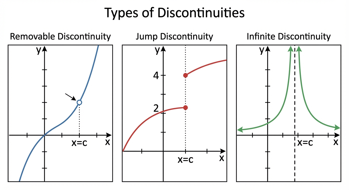
Types of Discontinuities
A function is continuous when its graph has no “breaks” in the sense that you can draw it without lifting your pencil (with an important caveat: continuity is a precise limit-based idea, not just a visual one). When a function is not continuous at some input value c, we say it has a discontinuity at c.
Understanding types of discontinuities matters because AP questions often ask you to (1) classify what kind of break is happening and (2) decide whether it can be fixed by redefining a value or adjusting a parameter. Different discontinuities come from different algebraic situations (holes, asymptotes, piecewise mismatches), and they behave differently with limits.
Removable discontinuity (a “hole”)
A removable discontinuity happens when:
- the limit exists and is finite, but
- is either undefined or not equal to that limit.
Visually, this often looks like a curve with a small open circle (a “hole”). Algebraically, it is usually caused by a common factor in the numerator and denominator of a rational function.
Example 1 (hole from canceling):
At x = 1 the expression is undefined, so does not exist.
Factor and simplify for x not equal to 1:
Now evaluate the limit:
So the limit exists and is finite, but the function is not defined at x = 1. That is a removable discontinuity at x = 1.
A key idea: you can “remove” this discontinuity by defining the missing value to equal the limit (this is developed fully in the “Removing Discontinuities” section).
Non-removable discontinuities
These are discontinuities that cannot be fixed by redefining a single point.
Jump discontinuity
A jump discontinuity happens when the one-sided limits both exist (and are finite), but they are not equal:
This is typical for piecewise-defined functions where the “pieces” do not meet. It also appears in absolute value–style definitions such as
Example 2 (piecewise mismatch):
Compute one-sided limits at c = 0:
They are not equal, so does not exist. This is a jump discontinuity at x = 0.
Because the two sides approach different y-values, no single choice of can make the function continuous there. This kind of discontinuity is not removable.
Infinite discontinuity (vertical asymptote)
An infinite discontinuity occurs when the function grows without bound near x = c. You’ll often see this in rational functions where the denominator goes to 0 and does not cancel.
You may describe it using one-sided behavior such as:
or
Example 3 (vertical asymptote):
As x approaches 2, the denominator approaches 0, so the function blows up:
The function has an infinite discontinuity at x = 2. This cannot be fixed by redefining because the function does not approach a finite value.
Oscillating discontinuity
An oscillating discontinuity is a rarer case where the function oscillates infinitely fast as it approaches a point, so the limit fails to exist due to oscillation rather than a jump or blow-up. A classic example is
at x = 0.
Discontinuities from domain restrictions (common sources)
Even when a question doesn’t ask you to “name the type,” you should be able to locate where continuity fails by checking where the function is not defined.
Common sources:
- Rational functions: denominator equals 0
- Even roots: square root requires the radicand to be at least 0 (in real-valued contexts)
- Logarithms: argument must be positive
- Piecewise functions: potential issues at boundary points
A frequent misconception is to say “the function is discontinuous where the denominator is zero.” That’s often true, but if a factor cancels, you may get a removable discontinuity (hole) instead of a vertical asymptote. You must check whether cancellation occurs.
Comparison table (discontinuity types)
| Type | Limit checklist failure | Visual characteristic |
|---|---|---|
| Removable | Condition 3 fails (limit does not equal the function value) | Hole in graph |
| Jump | Condition 2 fails (left-hand limit does not equal right-hand limit) | Vertical gap/step |
| Infinite | Condition 1 or 2 fails (function undefined or the “limit” is infinite) | Vertical asymptote |
Exam Focus
Typical question patterns
- Given a graph or formula, identify the x-values where f is discontinuous and classify each discontinuity (removable, jump, infinite, and occasionally oscillating).
- For a rational function, determine whether a discontinuity is a hole or a vertical asymptote by factoring and checking cancellation.
- For a piecewise function, compute one-sided limits at the boundary and decide whether the overall limit exists.
Common mistakes
- Concluding “removable” just because there is a discontinuity, without first verifying that exists and is finite.
- Forgetting that a jump discontinuity means the two one-sided limits are different (so the two-sided limit does not exist).
- Canceling factors and then incorrectly claiming the original function is defined at the canceled point.
- Assuming means vertical asymptote:
- If you get , that signals an infinite discontinuity (vertical asymptote).
- If you get , that strongly suggests a removable discontinuity (a hole) and you should factor first.
Confirming Continuity over an Interval
Saying “f is continuous” often means “f is continuous at every point in some interval.” This is more than a technical statement: continuity on an interval guarantees predictable behavior with no breaks, supports major theorems, and lets you use substitution-based limit evaluation throughout that interval.
Continuous on an open interval
A function f is continuous on the open interval if it is continuous at every point c with a < c < b. In practice, that means there are no holes, jumps, vertical asymptotes, or other breaks anywhere between a and b.
Continuous on a closed interval (endpoint one-sided continuity)
To claim continuity on a closed interval, you must be careful at the endpoints because a standard two-sided limit is not the relevant idea at an endpoint.
A function f is continuous on if:
- it is continuous on ,
- it is continuous from the right at a,
- it is continuous from the left at b.
In symbols:
![A graph of a function on a closed interval [a, b] showing solid dots at the endpoints to indicate continuity from the right at a and left at b.](https://knowt-user-attachments.s3.amazonaws.com/study-notes/8c4af29e-a7f7-4ae6-8ea3-14bc853d9775/039f4e77-0a91-4b69-83d2-ccc2a298c9c4.png)
Continuity of common function families (how you use it)
In AP Calculus AB, you are expected to know that many standard functions are continuous on their domains, which means you can confirm continuity quickly by checking where the function is defined.
- Polynomials are continuous for all real x.
- Rational functions are continuous wherever the denominator is not 0.
- Root functions (like square roots) are continuous wherever defined (for real outputs).
- Trigonometric functions: %%LATEX59%% and %%LATEX60%% are continuous for all real x; %%LATEX61%% is continuous wherever %%LATEX62%%.
- Exponential functions such as are continuous for all real x.
Example 1 (rational function: find intervals of continuity)
A rational function is continuous where it is defined, so find where the denominator is nonzero:
Factor:
So the denominator is 0 at x = 2 and x = -2. Therefore, f is continuous on:
A common mistake is to write or to include -2 or 2 in an interval. Continuity requires the function to be defined.
Example 2 (confirm continuity on a closed interval)
Is g continuous on ?
The domain condition is
so x must satisfy x ≥ 1. The entire interval %%LATEX74%% lies in the domain. Because the square root function is continuous where defined and %%LATEX75%% is continuous everywhere, their composition is continuous on its domain, so g is continuous on .
If the interval had been , you could not claim continuity on that closed interval because the function is not defined for inputs less than 1.
The Intermediate Value Theorem (IVT) as a continuity tool
One of the most testable “why continuity matters” results is the Intermediate Value Theorem:
If f is continuous on %%LATEX78%% and N is any number between %%LATEX79%% and %%LATEX80%%, then there exists at least one c in %%LATEX81%% such that
Interpretation: a continuous function cannot “skip” y-values between its endpoint values.
What IVT does and does not do:
- It guarantees existence of at least one solution.
- It does not give the exact value of c.
- It does not guarantee there is exactly one solution.
- It requires continuity on the entire interval.
Example 3 (use IVT to prove a root exists): Show that
has a solution in .
Let
Polynomials are continuous everywhere, so f is continuous on .
Evaluate endpoints:
Since 0 lies between -1 and 1, IVT guarantees some such that
So a root exists in .
Exam Focus
Typical question patterns
- “State the intervals on which f is continuous” for rational, root, exponential, trig, or piecewise functions.
- Determine whether f is continuous on (watch domain restrictions and the endpoint one-sided conditions).
- Use IVT to justify that a solution to exists in an interval by showing that k lies between endpoint values (often via a sign change when k = 0).
Common mistakes
- Forgetting that continuity on uses one-sided endpoint limits, not two-sided limits.
- Applying IVT when the function is not continuous on the entire interval (for example, a vertical asymptote inside the interval).
- Claiming IVT gives the value of the solution rather than just guaranteeing existence.
- Ignoring endpoints on closed intervals: trying to use two-sided limits at a or b instead of checking continuity only from within the interval.
Removing Discontinuities
Some discontinuities are “built in” and cannot be fixed (like vertical asymptotes or oscillations), but removable discontinuities can often be repaired by redefining the function at a point. On the AP exam, this appears in problems that ask you to “find a value of a constant that makes f continuous” or “define f(c) so that f becomes continuous at x = c.”
The guiding idea is simple: if you want continuity at x = c, the function value must match the limit.
The key rule for making a function continuous at a point
To make f continuous at x = c, you must ensure:
This only helps if the limit exists and is finite. If the limit does not exist (jump or oscillation) or is infinite (vertical asymptote), you cannot remove the discontinuity by choosing a value for .
Technique 1: Fixing a hole by redefining a single point
If a formula has a removable discontinuity at x = c (often because a factor cancels), then:
1) compute using algebraic simplification,
2) redefine the function at c to be L.
Example 1 (classic removable discontinuity fix):
For x not equal to 1, it simplifies to
and
To remove the discontinuity, define a new function F that matches the original everywhere except at x = 1:
Now F is continuous at x = 1.
A subtle but important point: simplifying %%LATEX103%% to %%LATEX104%% does not magically define the original function at x = 1. The “repair” happens only when you explicitly define the value at that point.
Technique 2: The algebraic approach (indeterminate form )
If evaluating a rational function’s limit gives the indeterminate form
there is likely a removable discontinuity caused by a common factor.
Worked Example: Let
Is there a discontinuity at x = 3? Can we remove it?
1) Check the function value:
So is undefined (Condition 1 fails).
2) Find the limit by factoring:
So for x not equal to 3,
Then
Since the limit exists and is finite, this is a removable discontinuity.
3) Redefine the function to plug the hole:
Now and
so g is continuous at x = 3.
Technique 3: Choosing a parameter to make a point continuous
AP problems often give a piecewise definition with an unknown constant at the problematic point. The continuity condition becomes an equation.
Example 2 (choose a constant for continuity): Find k so that f is continuous at x = 2.
Continuity requires
Factor:
So for x not equal to 2,
Then
What’s really happening: the “top rule” has a hole at x = 2, and you are choosing to plug the hole at exactly the limit height.
Technique 4: Continuity at a boundary in a general piecewise function (sometimes impossible)
Sometimes both pieces are already defined, and you must choose a constant that makes the left and right sides agree at the boundary. Occasionally, no value works.
Example 3 (match one-sided limits at a boundary): Find a so that f is continuous at x = 1.
Continuity at x = 1 requires the left-hand limit to equal the right-hand value:
Left-hand limit:
Right-hand value:
Set them equal:
Subtract a from both sides and you get an impossible statement (equivalently, 2 would have to equal 1). Therefore, no value of a makes f continuous at x = 1.
This is an important exam mindset: sometimes the correct conclusion is “continuity cannot be achieved,” not a numeric parameter value.
When discontinuities are not removable
It’s just as important to recognize when you cannot fix a discontinuity by redefining a point.
- Jump discontinuity: the two one-sided limits disagree, so there is no single y-value to assign.
- Infinite discontinuity: the function does not approach a finite value.
- Oscillating discontinuity: the function does not approach a single value due to oscillation.
A quick diagnostic: if %%LATEX129%% does not exist as a finite real number, you cannot remove the discontinuity at c by choosing %%LATEX130%%.
Exam Focus
Typical question patterns
- “Find k so that f is continuous at x = c” where k is the defined value at the point.
- “Find constants a and b so that f is continuous (and sometimes differentiable) at a boundary.” In this unit, continuity is the focus: match one-sided limits and function values.
- Identify whether a discontinuity is removable and, if so, define the missing value to remove it.
Common mistakes
- Setting %%LATEX131%% (or another random value) instead of using %%LATEX132%%.
- Forgetting to compute one-sided limits for piecewise functions (and assuming the two-sided limit exists).
- Trying to “fix” a vertical asymptote by choosing a value for even though the limit is infinite.
- Mixing up the key rational-function signals:
- suggests an infinite discontinuity (asymptote).
- suggests a removable discontinuity (hole), so factor and simplify.