Advanced Study Notes: Population Dynamics (APES Unit 3)
3.1 Generalist and Specialist Species
Ecological Range of Tolerance
Every species has a Range of Tolerance for abiotic conditions (temperature, humidity, salinity, pH). Within this range, there is an optimal zone where the species thrives.
Comparing Niches
Species are classified based on the breadth of their ecological niche and their ability to adapt to changing range conditions.
| Feature | Generalist Species | Specialist Species |
|---|---|---|
| Niche Width | Broad Niche | Narrow Niche |
| Resource Use | Can eat a variety of foods; broad habitat use | Specific dietary or habitat requirements |
| Environment | Thrives in changing/disrupted environments | Thrives in stable, constant environments |
| Advantage | High adaptability; less likely to go extinct during environmental stress | Less competition for their specific resources in stable conditions |
| Disadvantage | High competition for resources | Highly vulnerable to habitat loss or change |
| Examples | Humans, Raccoons, Cockroaches, Rats | Giant Pandas (bamboo), Koalas (eucalyptus), Salamanders |
Key Concept: When an ecosystem undergoes rapid change (e.g., climate change or urbanization), generalists generally fare better than specialists.
3.2 K-Selected and r-Selected Species
Reproductive strategies describe how species maximize their survival and reproductive success. These are often viewed on a spectrum (a continuum), but we categorize them into two extremes.
r-Selected Species (Biotic Potential Focus)
- "r" stands for: Growth rate (intrinsic rate of increase).
- Strategy: Produce as many offspring as possible in a short time.
- Goal: Quantity over quality.
- Characteristics:
- Small body size.
- Early maturity (reproduce young).
- Short life span.
- Little to no parental care.
- Boom-and-Bust cycles: Population shoots up quickly but crashes easily.
- Examples: Insects (mosquitoes), bacteria, algae, rodents, annual plants (dandelions).
K-Selected Species (Carrying Capacity Focus)
- "K" stands for: Carrying Capacity.
- Strategy: Invest heavily in a few offspring to ensure survival.
- Goal: Quality over quantity.
- Characteristics:
- Large body size.
- Late maturity (reproduce later in life).
- Long life span.
- High parental care (protection, teaching).
- Population stabilizes near carrying capacity.
- Examples: Humans, Elephants, Whales, Saguaro Cacti, Great Apes.
Invasive Species Connection
Most invasive species are r-selected generalists. Their high reproductive rate and lack of specific resource requirements allow them to outcompete native K-selected specialists.
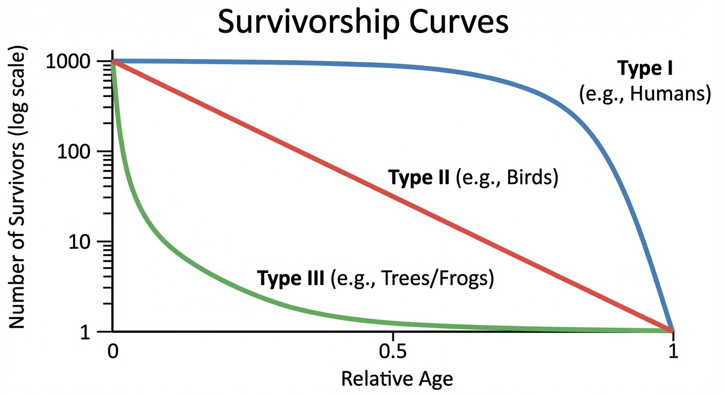
3.3 Survivorship Curves
A survivorship curve displays the relative survival rates of a cohort (a group of individuals of the same age) in a population, from birth to the maximum age reached.
The Three Types
Type I (Late Loss)
- Description: High survival throughout early and middle life; rapid decline in later life.
- Cause: High parental care and protection significantly reduce early mortality.
- Typical Species: K-selected species (Humans, Elephants, Primates).
Type II (Constant Loss)
- Description: Survival probabilities are roughly equal at all ages. The mortality rate is constant over the lifespan.
- Typical Species: Many birds, squirrels, rodents, reptiles, and some perennial plants.
Type III (Early Loss)
- Description: Very high mortality in early life; those few that survive the "bottleneck" tend to live long lives.
- Cause: Organisms produce thousands of offspring but provide no care. Predation is highest at the larval/seedling stage.
- Typical Species: r-selected species (Sea turtles, fish, oysters, insects, trees).
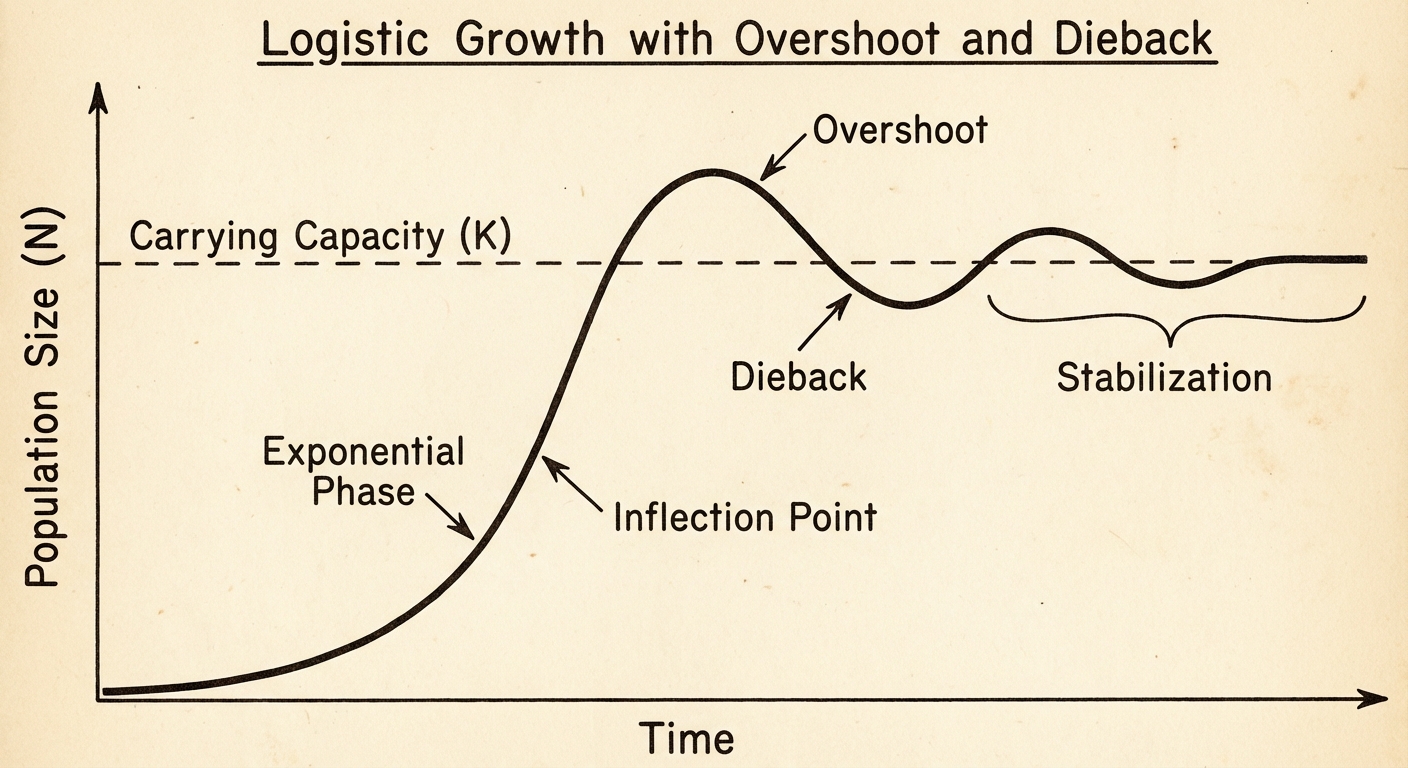
3.4 Carrying Capacity (K)
Definition
Carrying Capacity ($K$) is the maximum number of individuals of a population that a specific environment can sustain indefinitely given the available resources (food, water, space).
Overshoot and Dieback
- Overshoot: When a population grows beyond its carrying capacity ($N > K$). This usually happens because there is a reproductive time lag (gestation takes time).
- Dieback (Crash): Because the population has depleted its resources (famine, disease, competition), the population size decreases rapidly to fall back below $K$.
- consequence: Severe overshoot can degrade the resource base (e.g., overgrazing), permanently lowering the future carrying capacity.
3.5 Population Growth & Resource Availability
Population Growth Models
- Exponential Growth (J-Curve):
- Growth under ideal conditions with unlimited resources.
- Equation:
- No constraints on growth; strictly biotic potential.
- Logistic Growth (S-Curve):
- Growth that slows as the population approaches carrying capacity ($K$).
- Environmental resistance increases as density increases.
Limiting Factors
According to Liebig's Law of the Minimum, population growth is dictated not by the total resources available, but by the scarcest resource (the limiting factor).
| Density-Dependent Factors | Density-Independent Factors |
|---|---|
| Effect increases as population density rises. | Effect affects the population regardless of size. |
| Tend to be biotic (living). | Tend to be abiotic (non-living). |
| Competition for food/mates | Natural disasters (Floods, Fires, Hurricanes) |
| Disease / Parasitism | Severe weather / Climate change |
| Predation | Pollution / Pesticides |
| Accumulation of waste | Habitat destruction (Anthropogenic) |
3.6 Age Structure Diagrams (Population Pyramids)
These diagrams (histograms) show the distribution of various age groups in a population, usually separated by male and female.
Understanding Cohorts
- Prereproductive (0–14): Indicators of future growth.
- Reproductive (15–44): Determining current birth rates.
- Postreproductive (45+): Older generation.
Common Shapes & Interpretations
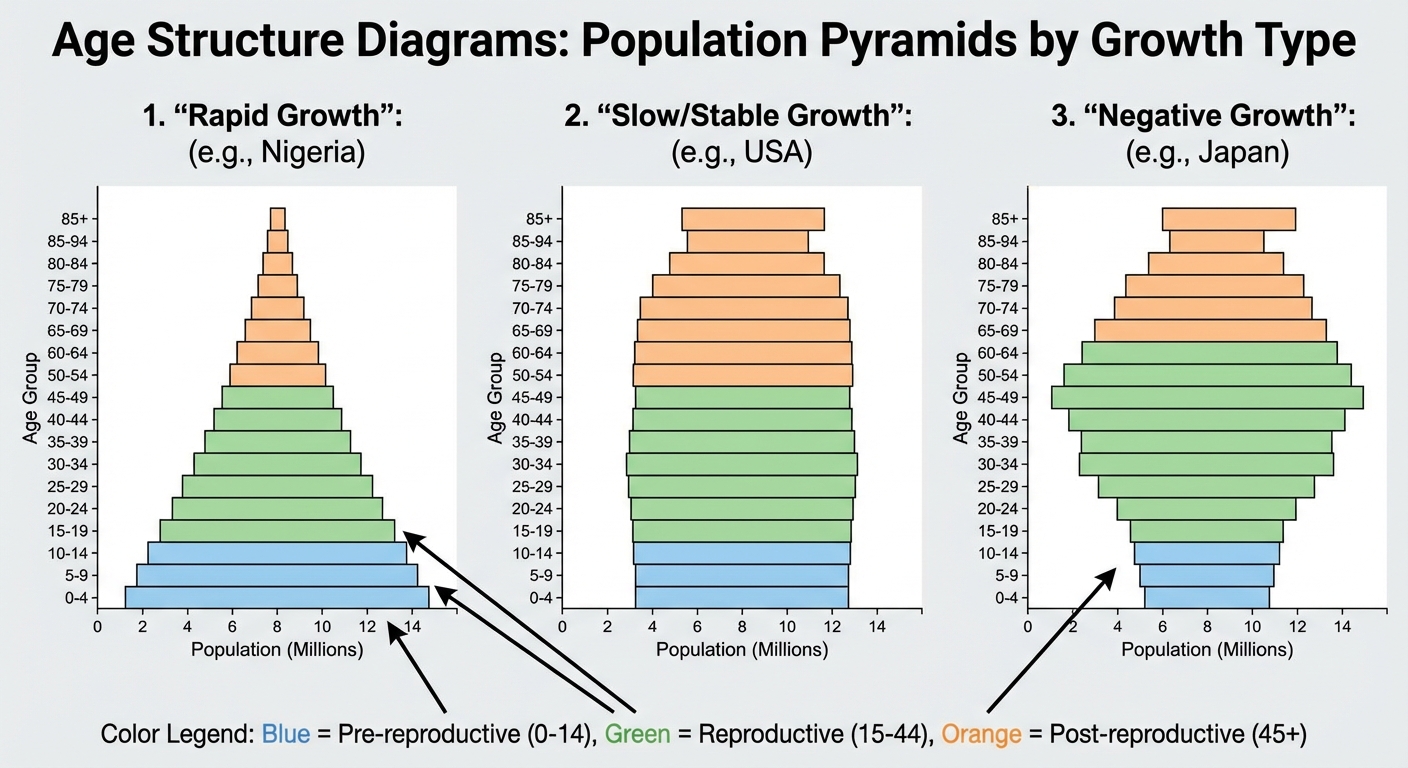
Broad Base (Triangle/Pyramid):
- Meaning: Rapid Population Growth.
- Why: Huge prereproductive cohort waiting to mature.
- Example: Nigeria, India, Guatemala.
Straight Sides (Column/Bell):
- Meaning: Stable/Slow Growth (Zero Population Growth - ZPG).
- Why: Birth rate $\approx$ Death rate.
- Example: USA, Canada, Australia.
Narrrow Base / Top Heavy (Inverted/Urn):
- Meaning: Declining Population (Negative Growth).
- Why: Fewer children are being born than people dying.
- Example: Japan, Germany, Russia, Italy.
Population Momentum: Even if fertility falls to replacement level, a population with a broad base will continue growing for a generation because there are so many young people entering reproductive age.
3.7 Total Fertility Rate (TFR)
Key Definitions
- Total Fertility Rate (TFR): The average number of children a woman will have in her lifetime.
- Global Average: $\approx 2.3$
- Developing: Higher TFR (allows for labor on farms, insurance for old age).
- Developed: Lower TFR (children are "economic liabilities" rather than assets).
- Replacement Level Fertility: The TFR required to keep a population size stable.
- Ideally 2.0, but actually 2.1 to account for infant mortality.
- In developing nations with high infant mortality, replacement level may be 2.5–3.0.
Factors Impacting TFR
- Education of Women: The single most significant factor. Educated women tend to marry later and have fewer, healthier children.
- Access to Contraception/Family Planning: Direct control over reproduction.
- Government Policies: Pro-natalist (e.g., tax breaks in France) vs. Anti-natalist (e.g., China's former One-Child Policy).
- Age of First Marriage: Delaying marriage reduces the fertile window utilized.
3.8 Human Population Dynamics & Math
Math: The Rule of 70
Estimates doubling time for exponential growth.
- Note: Keep $r$ as a percentage (e.g., for 2%, use 2, NOT 0.02).
- Example: A population growing at 2% doubles in $70/2 = 35$ years.
Standard Growth Formulas
- Growth Rate (r):
(Where CBR = Crude Birth Rate per 1,000 and CDR = Crude Death Rate per 1,000) - Population Density:
Malthusian Theory
- Thomas Malthus (1798): Predicted human population grows geometrically (exponentially) while food supply grows arithmetically (linearly).
- Result: Humans will hit a "Malthusian Catastrophe" (famine, war) unless checks limit population.
- Critique: He did not account for technological advancements (Green Revolution) increasing food yield density.
3.9 Demographic Transition Model (DTM)
The DTM explains how countries transition from high birth/death rates to low birth/death rates as they industrialize.
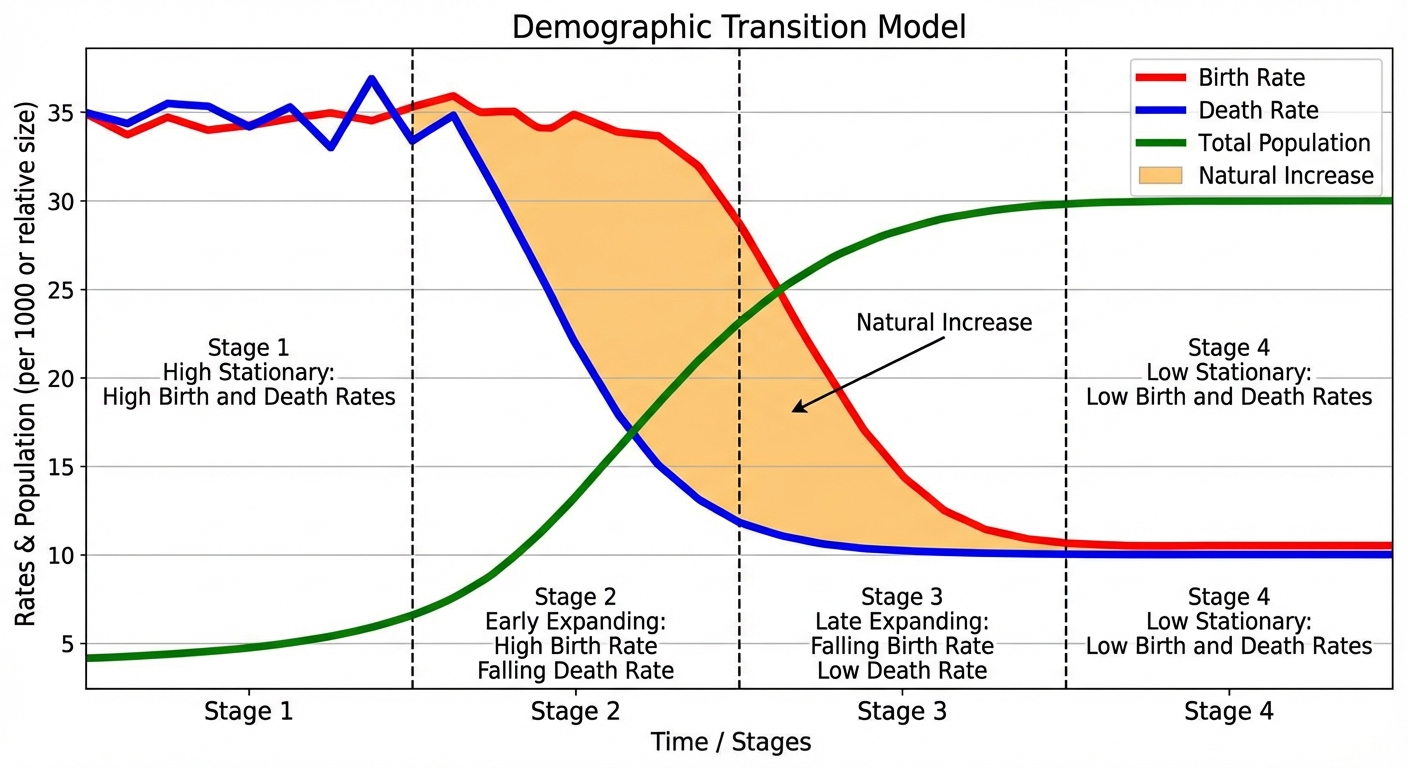
Stage 1: Pre-Industrial
- Birth Rate: High (Need farm labor, high infant mortality).
- Death Rate: High (Disease, famine, poor sanitation).
- Growth: Slow / Stable.
- Example: Very few distinct countries today; mostly remote tribal groups.
Stage 2: Transitional (Industrializing)
- Birth Rate: Remains High (Cultural lag—parents still think they need many kids).
- Death Rate: Plummets Rapidly (Introduction of modern medicine, sanitation, and clean water).
- Growth: Rapid / Exponential (This is where the population explosion happens).
- Example: Sub-Saharan Africa, Afghanistan.
Stage 3: Industrial
- Birth Rate: Starts to Fall Declining (Urbanization makes kids expensive; women enter workforce/education).
- Death Rate: Low and stable.
- Growth: Slowing down.
- Example: Mexico, India, Brazil.
Stage 4: Post-Industrial
- Birth Rate: Low (Equals death rate).
- Death Rate: Low.
- Growth: Zero Population Growth (ZPG) or stabilizing.
- Example: USA, UK, France.
Stage 5 (Theoretical): Declining
- Birth Rate: Drops below replacement level.
- Death Rate: Low, but may rise slightly due to an aging population.
- Growth: Negative.
- Example: Japan, Russia, Germany.
Common Mistakes & Pitfalls
- Confusing "r" and "K" selected with "r" (growth rate):
- Little "r" in math stands for growth rate. "r-selected" species are those that maximize this rate. Do not mix them up in free-response questions.
- Carrying Capacity is NOT constant:
- Students often draw K as a flat line. In reality, K changes if the environment changes (e.g., a drought lowers K; a new food source raises K).
- Density Dependent vs. Independent:
- Ask yourself: "Does the chance of dying increase if the crowd gets doubled?" If yes (e.g., flu transmission), it's dependent. If no (e.g., a tornado), it's independent.
- Math Errors in Rule of 70:
- Using the decimal (0.05) instead of the whole number (5). $70/0.05 = 1400$ years (WRONG) vs $70/5 = 14$ years (CORRECT).
- Demographic Transition Drivers:
- Remember that Death Rates fall FIRST (Stage 2), causing the boom. Birth rates only fall later (Stage 3). The population grows most when the gap between the two lines is widest.