AP Calculus BC Unit 7: Differential Equations (Slope Fields, Euler’s Method, Separable IVPs, Exponential and Logistic Models)

Understanding Differential Equations and Their Solutions

A differential equation is an equation that relates an unknown function (often written as

$y$

to one or more of its derivatives (like

$y'$

). In regular algebra, you usually solve for a number. In differential equations, you are solving for a function—a whole rule that describes how a quantity changes.

Differential equations connect naturally to earlier calculus ideas like related rates: in related rates, we modeled how one changing quantity is related to another using derivatives. Differential equations do something similar, except the “unknown” is the entire function whose rate of change is described.

The big idea is this: many real processes are easiest to describe by how they change moment-to-moment rather than by a direct formula. For example, “population increases at a rate proportional to the population” is naturally written in terms of a derivative.

Key vocabulary: order, solutions, and initial conditions

The order of a differential equation is the highest derivative that appears. For example,

$y' = x^2$

is first-order, while

$y'' + y = 0$

is second-order (not a major focus in this unit’s solving techniques).

A solution to a differential equation is a function that makes the equation true wherever it is defined. If you propose a function, you can verify it by substituting it into the differential equation and checking that both sides match.

A general solution is a family of solutions containing an arbitrary constant (often

$C$

). Many first-order differential equations have infinitely many solutions because you can shift the solution curve up or down.

An initial value problem (IVP) is a differential equation plus an initial condition like

$y(x_0)=y_0$

. The initial condition picks out one specific member of the family (a particular solution).

Why this matters: on the AP exam, a huge fraction of differential equation work is about interpreting what a differential equation is saying, approximating its solutions, and solving separable equations with an initial condition.

Notation you must recognize (they all mean “derivative”)

In AP Calculus BC, the same derivative may appear in different forms. You need to be fluent in switching between them.

A common misconception is to treat

$\frac{dy}{dx}$

as a simple fraction all the time. In general, it represents a derivative. But in separable differential equations, rewriting in “fraction-like” form is a powerful, valid technique.

What it means to solve (or not solve) a differential equation

There are three main outcomes you’ll see in this unit:

1. Solve exactly (usually via separation of variables): you find a formula for

$y$

(sometimes implicit).

2. Describe qualitatively: you sketch behavior from a slope field without an explicit formula.
3. Approximate numerically (Euler’s method): you compute approximate values of

$y$

at specified

$x$

-values.

Even when an exact solution exists, AP problems may still ask for numerical approximations or qualitative interpretations—because those skills mirror real applied work.

When “solving” is just antidifferentiating

If the differential equation gives the derivative of a function equal to a function of the independent variable alone, you can solve by integrating both sides. For example, if

$\frac{dy}{dx}=x^2$

then solving means finding an antiderivative:

$y=\int x^2\,dx$

which produces

$y=\frac{x^3}{3}+C$

This idea is part of the bigger theme: differential equation problems often involve “undoing a derivative.”

Exam Focus

• Typical question patterns:
  • “Verify that a given function is a solution to the differential equation, then use an initial condition to find the constant.”
  • “Given

$\frac{dy}{dx}$

determine whether a function is increasing/decreasing or concave up/down at a point.”

• “Interpret what the differential equation says about a real-world situation (units and meaning of terms).”
  • Common mistakes:
• Forgetting that solutions are functions (not single numbers), so you must include a constant in general solutions.
• Plugging into the differential equation incorrectly (especially mixing up

$y$

and

$y'$

).

• Treating an initial condition like

$y(0)=5$

as if it changes the differential equation itself—it only selects one solution.

Slope Fields and Qualitative Solution Behavior

A slope field (also called a direction field) is a picture that tells you the slope of solution curves at many points in the plane. Since a first-order differential equation gives

$y'$

as a function of

$x$

and

$y$

, it tells you the slope at every point

$(x,y)$

. A slope field visualizes that information.

Why this matters: many differential equations cannot be solved with elementary formulas, but you can still understand their behavior—where solutions rise, fall, level off, or approach equilibrium.

How to construct a slope field (mechanics)

To construct a slope field, you plug the point’s coordinates into the differential equation to get the slope at that point, then draw a small line segment with that slope. In other words: evaluate the right-hand side at the point and draw that as the slope.

For example, for the equation

$\frac{dy}{dx}=x$

the slope depends only on

$x$

. So at

$x=-1$

the slope is

$-1$

no matter what

$y$

is.

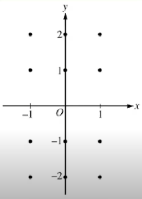
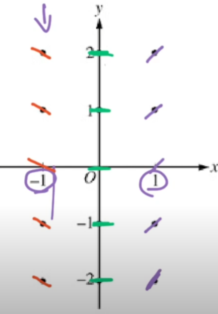
How to read a slope field

If you have a differential equation

$\frac{dy}{dx}=F(x,y)$

then at each point

$(x,y)$

the slope of the solution curve is

$F(x,y)$

.

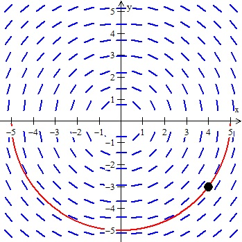
To sketch solution curves:

• Pick a starting point (often an initial condition).
• Follow the little line segments, drawing a smooth curve that is always tangent to the segment directions.

When the AP exam asks for a solution curve from a slope field, the core skill is to “flow” with the slopes. Because this is by hand, it doesn’t have to be exact, but it should consistently track the tangent directions.

Two important clarifications:

• Solution curves cannot cross (in typical AP settings where

$F(x,y)$

is well-behaved). If they crossed, you would have two different slopes at the same point, which contradicts the idea that the differential equation assigns a unique slope.

• A slope field gives local information (slope at a point), not a direct formula for the entire curve.

Isoclines: places where the slope is constant

An isocline is a curve where the slope

$\frac{dy}{dx}$

has a constant value

$k$

:

$F(x,y)=k$

On a slope field, isoclines help you organize the picture: along that curve, all the direction segments have the same slope. You won’t always be asked to find isoclines, but the idea helps you reason about patterns.

Equilibrium solutions (constant solutions)

An equilibrium solution is a constant solution

$y=c$

such that the derivative is zero everywhere along that horizontal line. For equations of the form

$\frac{dy}{dx}=G(y)$

equilibria occur when

$G(c)=0$

These matter especially for autonomous differential equations (where the right side depends only on

$y$

). Equilibrium solutions often represent steady states like a stabilized population.

Stability intuition (qualitative)

If nearby solutions move toward an equilibrium as

$x$

increases, it’s stable. If nearby solutions move away, it’s unstable. You can often decide this by checking the sign of

$G(y)$

above and below the equilibrium.

Worked example: sketching behavior from a differential equation

Suppose

$\frac{dy}{dx}=y(1-y)$

This is an autonomous equation. Look for equilibria:

$y(1-y)=0$

So equilibria are

$y=0$

and

$y=1$

Now analyze the sign of

$y(1-y)$

:

• If

$0<y<1$

, then

$y>0$

and

$1-y>0$

, so

$y' > 0$

. Solutions increase.

• If

$y>1$

, then

$1-y<0$

, so

$y' < 0$

. Solutions decrease.

• If

$y<0$

, then

$y<0$

and

$1-y>0$

, so

$y' < 0$

. Solutions decrease further.

Conclusion: solutions between 0 and 1 rise toward 1; solutions above 1 fall toward 1. So

$y=1$

is stable, and

$y=0$

is unstable.

This kind of reasoning shows up often: you may not need an explicit solution to predict long-term behavior.

Exam Focus

• Typical question patterns:
  • “Use the slope field to sketch the solution satisfying

$y(x_0)=y_0$

.”

• “From the slope field, estimate

$y(x)$

at a given

$x$

.”

• “Identify equilibrium solutions and determine stability from sign analysis or the slope field.”
  • Common mistakes:
• Drawing solution curves that follow the small segments but aren’t smooth or that kink sharply—solutions should look like smooth curves.
• Forgetting that the slope at a point depends on both coordinates (students sometimes use only

$x$

or only

$y$

without checking the equation).

• Misidentifying equilibria by setting

$y'=0$

incorrectly (especially when the right side is factored).

• Crossing abruptly or drawing a curve that does not follow the indicated slopes when sketching by hand.

Euler’s Method: Approximating Solutions Numerically

Even if you can’t solve a differential equation symbolically, you can still approximate its solution values. Euler’s method is the main numerical approximation technique in AP Calculus.

Conceptually, Euler’s method takes the differential equation’s message—“the slope at this point is

$y'$

”—and uses that slope to step forward in small increments. It’s like repeatedly using the tangent line as a local approximation.

The core idea: tangent line stepping

Given an IVP

$\frac{dy}{dx}=F(x,y)$

with an initial point

$(x_0,y_0)$

, choose a step size

$h$

. Euler’s method produces points

$(x_n,y_n)$

via

$x_{n+1}=x_n+h$

and

$y_{n+1}=y_n+hF(x_n,y_n)$

Why this formula makes sense: over a small step

$h$

, the change in

$y$

is approximately slope times run. The slope at the start of the interval is

$F(x_n,y_n)$

, so

$\Delta y\approx F(x_n,y_n)h$

A common misunderstanding is to think Euler’s method uses the slope at the end of the interval. Standard Euler uses the slope at the beginning of each step.

How AP problems structure Euler’s method

You might be given:

• the differential equation,
• an initial condition,
• a step size (like

$h=0.2$

),

• and asked to find

$y$

at a certain

$x$

after a few steps.

Sometimes, AP will provide a table with values of

$F(x,y)$

so that you can compute without repeatedly plugging into a formula.

Worked example: 3 Euler steps

Approximate the solution to

$\frac{dy}{dx}=x+y$

with

$y(0)=1$

using step size

$h=0.5$

to estimate

$y(1.5)$

.

Start:

$x_0=0$

$y_0=1$

Step 1 to

$x_1=0.5$

:

$y_1=y_0+h(x_0+y_0)$

$y_1=1+0.5(0+1)=1.5$

Step 2 to

$x_2=1.0$

:

$y_2=y_1+0.5(x_1+y_1)$

$y_2=1.5+0.5(0.5+1.5)=2.5$

Step 3 to

$x_3=1.5$

:

$y_3=y_2+0.5(x_2+y_2)$

$y_3=2.5+0.5(1+2.5)=4.25$

So Euler’s method gives

$y(1.5)\approx 4.25$

Error and step size (what you should understand)

Euler’s method is an approximation. The key control you have is the step size

$h$

.

• Smaller

$h$

typically improves accuracy because the tangent-line approximation is more valid over shorter intervals.

• Larger

$h$

can accumulate significant error.

There are two useful ideas about error that AP-level intuition often tests:

1. Local truncation error: the error made in a single step.
2. Global error: the accumulated error after many steps.

You are rarely asked to compute an exact error bound in this unit, but you should be able to explain qualitatively that decreasing

$h$

tends to reduce error.

Also, Euler’s method can under- or over-estimate depending on the solution’s concavity. If the true solution is concave up, tangent lines tend to lie below the curve, often making Euler an underestimate (and vice versa for concave down). This is a helpful heuristic, not a guarantee in every scenario.

Exam Focus

• Typical question patterns:
  • “Use Euler’s method with step size

$h$

to approximate

$y(x)$

after

$n$

steps.”

• “Given a table of slopes, use Euler’s method to approximate the solution.”
• “Compare two Euler approximations with different step sizes and comment on which is more accurate.”
  • Common mistakes:
• Using the wrong point to evaluate slope, such as

$F(x_{n+1},y_{n+1})$

instead of

$F(x_n,y_n)$

.

• Mixing up step size with number of steps (for example, stepping from

$0$

to

$2$

with

$h=0.5$

requires 4 steps).

• Arithmetic drift: small arithmetic errors compound; writing a clean table of

$x_n$

,

$y_n$

, and slope helps.

Separable Differential Equations and Solving Initial Value Problems

A separable differential equation is a first-order differential equation that can be rearranged so that all

$y$

terms are on one side and all

$x$

terms are on the other. This is the main exact-solving technique emphasized in AP Calculus BC for differential equations.

A memory checklist: SIPPY

A useful memory trick is that many separable differential equation IVP problems follow the steps SIPPY:

• S: separate (get

$dy$

and

$dx$

on separate sides)

• I: integrate (remove the derivative)
• P: plus

$C$

(add your constant of integration)

• P: plug in your initial condition
• Y: solve so “

$y$

equals …” (make

$y$

explicit when appropriate)

What “separable” means

A common separable form is

$\frac{dy}{dx}=f(x)g(y)$

The goal is to rewrite it as

$\frac{1}{g(y)}\,dy=f(x)\,dx$

Then you integrate both sides:

$\int \frac{1}{g(y)}\,dy=\int f(x)\,dx$

This works because (in this context) you can treat

$dy$

and

$dx$

as differentials that “travel” with their variables. A good way to stay grounded is to remember that you are applying a chain rule idea in reverse: if

$y$

depends on

$x$

, then integrating with respect to

$y$

on one side and

$x$

on the other can produce a relationship between them.

The constant of integration and where it goes

After integrating, you must include a constant. You might see constants on both sides; you can always combine them into a single constant.

For example,

$\int \frac{1}{g(y)}\,dy=\int f(x)\,dx$

becomes

$H(y)=G(x)+C$

A very common student error is forgetting

$C$

entirely, or putting separate constants and never combining them.

Implicit vs explicit solutions

Often you will end with an implicit solution (an equation involving both

$x$

and

$y$

). Sometimes you can solve for

$y$

explicitly; sometimes it’s messy or unnecessary.

AP will accept implicit solutions in many contexts, especially when the focus is on applying an initial condition or analyzing behavior.

Worked example 1: solve a separable DE (general solution)

Solve

$\frac{dy}{dx}=x y$

Separate variables:

$\frac{1}{y}\,dy=x\,dx$

Integrate:

$\int \frac{1}{y}\,dy=\int x\,dx$

So

$\ln |y|=\frac{x^2}{2}+C$

Exponentiate both sides:

$|y|=e^{\frac{x^2}{2}+C}$

Rewrite

$e^C$

as a new positive constant

$K$

:

$|y|=Ke^{\frac{x^2}{2}}$

To allow negative solutions too, fold the sign into a single nonzero constant

$A$

:

$y=Ae^{\frac{x^2}{2}}$

That is the general solution.

Worked example 2: initial value problem

Solve the IVP

$\frac{dy}{dx}=x y$

$y(0)=3$

From the general solution:

$y=Ae^{\frac{x^2}{2}}$

Apply the initial condition:

$3=Ae^0$

So

$A=3$

Therefore the particular solution is

$y=3e^{\frac{x^2}{2}}$

Worked example 3 (SIPPY in action): an IVP with algebra at the end

Solve

$\frac{dy}{dx}=\frac{4x}{y}$

with

$y(0)=5$

Separate by multiplying both sides by

$y\,dx$

:

$y\,dy=4x\,dx$

Integrate:

$\int y\,dy=\int 4x\,dx$

which gives

$\frac{y^2}{2}=2x^2+C$

Plug in the initial condition:

$\frac{5^2}{2}=2\cdot 0^2 + C$

So

$C=\frac{25}{2}$

Now substitute back:

$\frac{y^2}{2}=2x^2+\frac{25}{2}$

Multiply both sides by 2:

$y^2=4x^2+25$

Finally, solve for

$y$

:

$y=\pm\sqrt{4x^2+25}$

Use

$y(0)=5$

to choose the positive branch, so the particular solution is

$y=\sqrt{4x^2+25}$

Important pitfall to avoid: from

$\frac{y^2}{2}=2x^2+\frac{25}{2}$

it is incorrect to conclude

$y=2x^2+\frac{25}{2}$

That mistake comes from “taking the square root” incorrectly (you must isolate

$y^2$

first, then take the square root).

Handling algebra carefully (a common pitfall)

When separating variables, you must divide by expressions involving

$y$

or

$x$

. That can accidentally exclude solutions.

Example: if you divide by

$y$

, you assume

$y\neq 0$

. But sometimes

$y=0$

is actually a solution (an equilibrium solution). In the earlier equation

$y'=xy$

, note that

$y=0$

does satisfy it, so it should be included as an additional solution.

A safe habit: after solving, quickly check whether any constant solutions (like

$y=0$

) were lost when dividing.

Using definite integrals to apply initial conditions cleanly

Sometimes it’s cleaner to integrate with limits immediately, especially in AP free-response.

If

$y(x_0)=y_0$

, you can write

$\int_{y_0}^{y} \frac{1}{g(u)}\,du=\int_{x_0}^{x} f(t)\,dt$

This automatically builds in the initial condition and avoids the “where do I put

$C$

?” issue.

Exam Focus

• Typical question patterns:
  • “Solve the differential equation by separation of variables and use an initial condition to find the particular solution.”
  • “Find the solution implicitly and then evaluate

$y$

at a given

$x$

.”

• “Show that the solution satisfies the differential equation (differentiate your solution and substitute).”
  • Common mistakes:
• Separating incorrectly (for example, moving terms but forgetting parentheses or factors).
• Losing solutions by dividing by a variable expression (especially missing equilibrium solutions).
• Applying the initial condition to an implicit equation incorrectly (substitute

$x_0$

and

$y_0$

carefully, then solve for the constant).

• Forgetting

$C$

(“Plus C”) after integrating.

Exponential Growth and Decay Models from Differential Equations

Exponential models in calculus come from a simple but powerful assumption: the rate of change of a quantity is proportional to the amount present.

The proportionality differential equation

If a quantity

$y$

changes at a rate proportional to its current value, then

$\frac{dy}{dx}=ky$

where

$k$

is a constant of proportionality.

• If

$k>0$

, you get exponential growth.

• If

$k<0$

, you get exponential decay.

This model appears in populations (unlimited resources), continuously compounded interest, certain chemical reactions, and radioactive decay.

Solving the model (and why the result is exponential)

Separate variables:

$\frac{1}{y}\,dy=k\,dx$

Integrate:

$\ln |y|=kx+C$

Exponentiate:

$y=Ae^{kx}$

where

$A$

is a nonzero constant (and can be determined from an initial condition). If you know

$y(0)=y_0$

, then

$A=y_0$

.

So the typical IVP solution is

$y=y_0e^{kx}$

A conceptual note: the fact that you get

$e^{kx}$

is not arbitrary—

$e^x$

is the unique function whose derivative is proportional to itself.

Doubling time and half-life

For growth, the doubling time

$T$

satisfies

$2y_0=y_0e^{kT}$

So

$2=e^{kT}$

Take natural log:

$\ln 2=kT$

Thus

$T=\frac{\ln 2}{k}$

For decay, the half-life

$T$

satisfies

$\frac{1}{2}y_0=y_0e^{kT}$

So

$\frac{1}{2}=e^{kT}$

Take natural log:

$\ln \left(\frac{1}{2}\right)=kT$

Thus

$T=\frac{\ln(1/2)}{k}$

Since

$k<0$

for decay, this gives a positive half-life.

Worked example: determine $k$ from data

A bacteria culture grows according to

$\frac{dy}{dt}=ky$

. If

$y(0)=500$

and

$y(3)=800$

, find

$k$

and the model.

General solution:

$y=500e^{kt}$

Use

$y(3)=800$

:

$800=500e^{3k}$

Divide:

$\frac{8}{5}=e^{3k}$

Take ln:

$\ln \left(\frac{8}{5}\right)=3k$

So

$k=\frac{1}{3}\ln \left(\frac{8}{5}\right)$

Model:

$y=500e^{\left(\frac{1}{3}\ln(8/5)\right)t}$

A common mistake here is to write

$k=\ln(8/5)$

and forget to divide by 3.

Interpreting $k$ with units

If

$t$

is measured in days, then

$k$

has units of “per day.” This matters: it tells you how fast exponential growth/decay is happening relative to the time variable.

Exam Focus

• Typical question patterns:
  • “Given ‘rate proportional to amount,’ write a differential equation and solve for

$y(t)$

.”

• “Use two points on the curve to find

$k$

, then predict a future value.”

• “Find doubling time or half-life using the differential equation model.”
  • Common mistakes:
• Using the wrong initial condition time (for example, treating

$y(2)=y_0$

as if it were

$y(0)=y_0$

without shifting appropriately).

• Confusing linear and exponential change (constant rate versus rate proportional to amount).
• Sign errors: forgetting that decay corresponds to

$k<0$

.

Logistic Differential Equations: Growth with a Carrying Capacity

Pure exponential growth is often unrealistic for long periods because it assumes unlimited resources. The logistic model modifies exponential growth by building in a limiting factor: as the population gets large, the growth rate slows.

The logistic differential equation

A standard logistic model for a population

$P$

is

$\frac{dP}{dt}=rP\left(1-\frac{P}{K}\right)$

where:

$r$

is the intrinsic growth rate (per unit time).

$K$

is the carrying capacity (the maximum sustainable population).

Interpretation of the factor:

• When

$P$

is small relative to

$K$

, the factor

$\left(1-\frac{P}{K}\right)$

is close to 1, and growth is approximately exponential:

$P'\approx rP$

• When

$P$

approaches

$K$

, the factor approaches 0, so growth slows.

• If

$P>K$

, the factor becomes negative, making

$P'<0$

, so the population decreases back toward

$K$

.

This differential equation is a major AP topic because it combines modeling, equilibrium analysis, and separable solving.

Equilibria and long-term behavior

Set

$\frac{dP}{dt}=0$

:

$rP\left(1-\frac{P}{K}\right)=0$

Equilibria:

$P=0$

and

$P=K$

Stability reasoning (assuming

$r>0$

):

• If

$0<P<K$

, then

$P'>0$

, so solutions increase.

• If

$P>K$

, then

$P'<0$

, so solutions decrease.

So

$P=K$

is stable, and

$P=0$

is unstable (in the model).

Solving the logistic equation (separation of variables)

Start with

$\frac{dP}{dt}=rP\left(1-\frac{P}{K}\right)$

Rewrite the factor:

$1-\frac{P}{K}=\frac{K-P}{K}$

So

$\frac{dP}{dt}=\frac{r}{K}P(K-P)$

Separate variables:

$\frac{1}{P(K-P)}\,dP=\frac{r}{K}\,dt$

To integrate the left side, you use partial fractions:

$\frac{1}{P(K-P)}=\frac{1}{K}\left(\frac{1}{P}+\frac{1}{K-P}\right)$

Integrate:

$\int \frac{1}{P(K-P)}\,dP=\int \frac{r}{K}\,dt$

So

$\frac{1}{K}\int \left(\frac{1}{P}+\frac{1}{K-P}\right)dP=\frac{r}{K}t+C$

Compute integrals (note that

$\int \frac{1}{K-P}dP=-\ln|K-P|$

):

$\frac{1}{K}\left(\ln|P|-\ln|K-P|\right)=\frac{r}{K}t+C$

Multiply by

$K$

:

$\ln\left|\frac{P}{K-P}\right|=rt+C$

Exponentiate:

$\left|\frac{P}{K-P}\right|=Ae^{rt}$

For the typical population setting with

$0<P<K$

, you can drop absolute values and write

$\frac{P}{K-P}=Ae^{rt}$

Solve for

$P$

:

$P=Ae^{rt}(K-P)$

$P=AKe^{rt}-Ae^{rt}P$

$P+Ae^{rt}P=AKe^{rt}$

$P(1+Ae^{rt})=AKe^{rt}$

$P=\frac{AKe^{rt}}{1+Ae^{rt}}$

A common equivalent form is obtained by dividing numerator and denominator by

$Ae^{rt}$

:

$P=\frac{K}{1+Be^{-rt}}$

where

$B=\frac{1}{A}$

.

Worked example: use an initial condition

Suppose

$K=1000$

and

$r=0.4$

, and

$P(0)=200$

. Find

$P(t)$

.

Use the form

$P=\frac{K}{1+Be^{-rt}}$

Substitute

$t=0$

:

$200=\frac{1000}{1+B}$

So

$1+B=5$

Thus

$B=4$

Therefore

$P(t)=\frac{1000}{1+4e^{-0.4t}}$

This model clearly shows the long-term behavior: as

$t\to \infty$

,

$e^{-0.4t}\to 0$

, and

$P(t)\to 1000$

.

The inflection point (where growth is fastest)

In the logistic model, the population grows fastest at half the carrying capacity:

$P=\frac{K}{2}$

That corresponds to the inflection point of the logistic curve (where it switches from concave up to concave down). You may be asked to interpret this: early on, growth accelerates; later, growth slows as resources become limiting.

Exam Focus

• Typical question patterns:
  • “Write a logistic differential equation from a description involving carrying capacity.”
  • “Find equilibrium solutions and determine stability.”
  • “Solve the logistic differential equation (often with an initial condition) and interpret long-term behavior.”
• Common mistakes:
  • Mixing up

$K$

and

$r$

:

$K$

sets the horizontal asymptote;

$r$

controls how quickly the curve approaches it.

• Algebra errors when solving for

$P$

after exponentiating (losing track of constants like

$A$

and

$B$

).

• Forgetting that

$P=0$

and

$P=K$

are solutions even if you proceed by dividing by

$P(K-P)$

.

Building Differential Equations from Context and Interpreting Solutions

On AP free-response, you are often not handed a “nice” differential equation first. Instead, you’re given a situation, and you must model it with a differential equation, interpret what the model predicts, and sometimes approximate or solve.

Translating words into a differential equation

Here are common phrases and the differential equation structures they suggest:

1) “Rate is proportional to amount”

$\frac{dy}{dt}=ky$

2) “Rate is proportional to the product of the amount and the remaining capacity” (logistic)

$\frac{dP}{dt}=rP\left(1-\frac{P}{K}\right)$

3) “Rate depends on both time and current amount”

$\frac{dy}{dt}=F(t,y)$

In any modeling situation, take a moment to label:

• what the independent variable represents (often time),
• what the dependent variable represents (population, temperature, mass, etc.),
• and the units of the derivative.

Units as a consistency check

A powerful way to avoid mistakes is to track units.

• If

$y$

is measured in liters and

$t$

in minutes, then

$\frac{dy}{dt}$

is liters per minute.

• In

$\frac{dy}{dt}=ky$

, the constant

$k$

must have units of “per minute,” because multiplying “per minute” by liters gives liters per minute.

If your units don’t match, your model (or algebra) is wrong.

Interpreting a derivative at a point

If you are given

$\frac{dy}{dx}=F(x,y)$

and a point

$(a,b)$

on a solution curve, then

$y'(a)=F(a,b)$

This tells you the instantaneous rate of change at that point. AP loves asking for interpretations like: “At time

$t=a$

, the population is increasing at

$F(a,b)$

organisms per day.”

Using the second derivative to infer concavity (without solving)

Sometimes you’re asked whether a solution is concave up or down at a point, given only

$y'=F(x,y)$

.

You can differentiate implicitly:

$y''=\frac{d}{dx}F(x,y)$

If

$F$

depends on

$y$

, you must apply the chain rule. For example, if

$y'=x-y$

then

$y''=1-y'$

because the derivative of

$-y$

is

$-y'$

.

Then at a point

$(a,b)$

you can compute

$y'(a)$

first, then plug into

$y''(a)$

.

Worked example: concavity from a differential equation

Given

$\frac{dy}{dx}=x-y$

and a solution passing through

$(2,1)$

, determine whether it is concave up or down at

$x=2$

.

First compute the slope at the point:

$y'(2)=2-1=1$

Differentiate to find

$y''$

:

$y''=\frac{d}{dx}(x-y)=1-y'$

Evaluate at

$x=2$

:

$y''(2)=1-y'(2)=1-1=0$

So at

$x=2$

the concavity test is inconclusive from this value alone:

$y''(2)=0$

means the curve is neither concave up nor concave down at that instant (it could be an inflection point, or just a flat change in concavity). Many students incorrectly conclude “concave up” when they see 0; the correct conclusion is that concavity is not up or down at that exact point.

When you should not try to solve

AP problems sometimes place you in a setting where separation is not feasible, such as

$\frac{dy}{dx}=x+y^2$

This is not separable in a useful way for elementary functions. In those cases, tasks usually shift to:

• evaluating

$y'$

at a point,

• using Euler’s method,
• using a slope field,
• or analyzing sign and behavior.

Recognizing when to stop trying to separate is a real exam skill.

Exam Focus

• Typical question patterns:
  • “Write a differential equation that models the situation; identify what each term means.”
  • “Given

$y'=F(x,y)$

and

$y(a)=b$

, find

$y'(a)$

and interpret it in context.”

• “Use the differential equation to determine where the solution is increasing/decreasing or concave up/down.”
  • Common mistakes:
• Ignoring units and interpreting a rate with the wrong units (e.g., saying ‘people’ instead of ‘people per year’).
• Computing

$y''$

and forgetting the chain rule term involving

$y'$

.

• Trying to separate a non-separable equation and producing invalid algebra.

Differential Equations on AP Free-Response: Multi-Representation Tasks

Differential equations frequently appear in AP free-response questions that combine multiple representations: a differential equation, a table, a slope field, and/or a graph. The exam often wants you to connect these views rather than only “solve.”

Moving between an equation, a table, and an approximation

You might be given a table of values of

$F(x,y)$

for a differential equation

$y'=F(x,y)$

. This is common when the function is complicated or when the exam wants to emphasize numerical reasoning.

If you have Euler’s method with step size

$h$

:

$y_{n+1}=y_n+hF(x_n,y_n)$

and a table provides

$F(x_n,y_n)$

directly, you can compute successive values without algebraic substitution.

A key habit: always record the triple

$x_n$

,

$y_n$

, and slope

$F(x_n,y_n)$

so you can see what you used at each step.

Estimating a solution value from a slope field

If asked to estimate

$y(b)$

given

$y(a)=c$

, you trace the solution curve across the slope field from

$x=a$

to

$x=b$

. Because this is approximate, your accuracy depends on careful tracing and reading the axes.

Two common pitfalls:

• drifting off the direction segments (your curve must stay tangent to them),
• forgetting that different solution curves correspond to different initial conditions.

Checking reasonableness: monotonicity and asymptotes

Even when you do compute or estimate a value, AP often expects a “reasonableness check.” For example:

• If slopes are positive along the path, your solution should be increasing.
• If the model is logistic with carrying capacity

$K$

, your values should not blow past

$K$

and keep increasing forever (unless the initial condition is above

$K$

, in which case it should decrease).

Being able to say “this answer makes sense because the slope field shows decreasing slopes” can earn explanation points.

Worked example: combining separation and interpretation

A tank contains a salt solution. Let

$S(t)$

be the amount of salt (in grams). Suppose it follows

$\frac{dS}{dt}=-0.2S$

and

$S(0)=50$

.

1) Solve for

$S(t)$

.

This is exponential decay:

$S=50e^{-0.2t}$

2) Interpret

$S'(3)$

.

First find

$S(3)$

:

$S(3)=50e^{-0.6}$

Then compute the derivative from the differential equation:

$S'(3)=-0.2S(3)$

So

$S'(3)=-0.2\cdot 50e^{-0.6}=-10e^{-0.6}$

Interpretation: at

$t=3$

(units of time), the amount of salt is decreasing at a rate of

$10e^{-0.6}$

grams per unit time.

Notice the exam strategy: you do not need to differentiate

$S(t)$

again; the differential equation already tells you

$S'$

in terms of

$S$

.

Exam Focus

• Typical question patterns:
  • “Use a table of values of

$y'$

with Euler’s method to approximate

$y$

.”

• “Estimate

$y(b)$

from a slope field given an initial condition.”

• “Solve a separable differential equation, then use the model to interpret a rate at a specific time.”
  • Common mistakes:
• Treating slope-field estimates as exact (they are approximate, so answers should be written as estimates).
• Forgetting that you can often compute

$y'(a)$

directly from

$y'=F(x,y)$

without finding

$y(x)$

.

• Losing track of what the dependent variable represents (amount of salt versus concentration, for example).