AP Precalculus Unit 2: Exponential Functions Mastery Guide
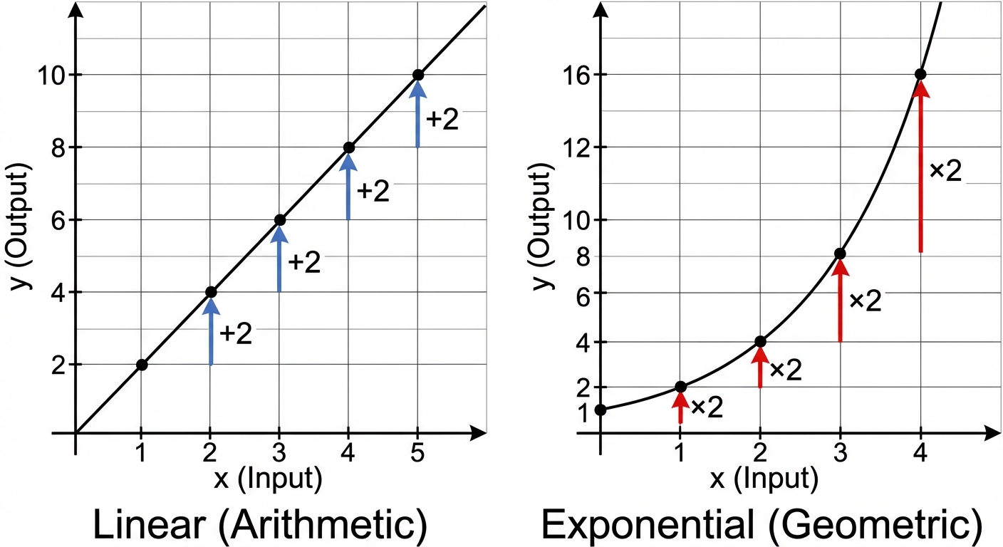
Arithmetic and Geometric Sequences
Before diving into continuous exponential functions, AP Precalculus establishes the foundation using discrete sequences. Understanding the pattern of change in sequences is critical for identifying function types.
Definitions & Patterns
There are two primary ways sequences change over equal intervals:
Arithmetic Sequences
- Definition: A sequence where each term is generated by adding a constant value to the previous term.
- Key Characteristic: Constant common difference ($d$).
- Function Connection: Models Linear Functions ($y = mx + b$).
Geometric Sequences
- Definition: A sequence where each term is generated by multiplying the previous term by a constant non-zero value.
- Key Characteristic: Constant common ratio ($r$).
- Function Connection: Models Exponential Functions ($y = a \cdot b^x$).
Formulas and Notation
| Feature | Arithmetic Sequence | Geometric Sequence |
|---|---|---|
| Recursive Rule | $un = u{n-1} + d$ | $un = u{n-1} \cdot r$ |
| Explicit Rule | $un = u0 + n \cdot d$ | $un = u0 \cdot r^n$ |
| Associated Function | Linear: $f(x) = b + mx$ | Exponential: $f(x) = a \cdot b^x$ |
| Change Type | Additive Change | Multiplicative Change |
Key Concept: In an arithmetic sequence, successive terms have a constant difference. In a geometric sequence, successive terms have a constant ratio.
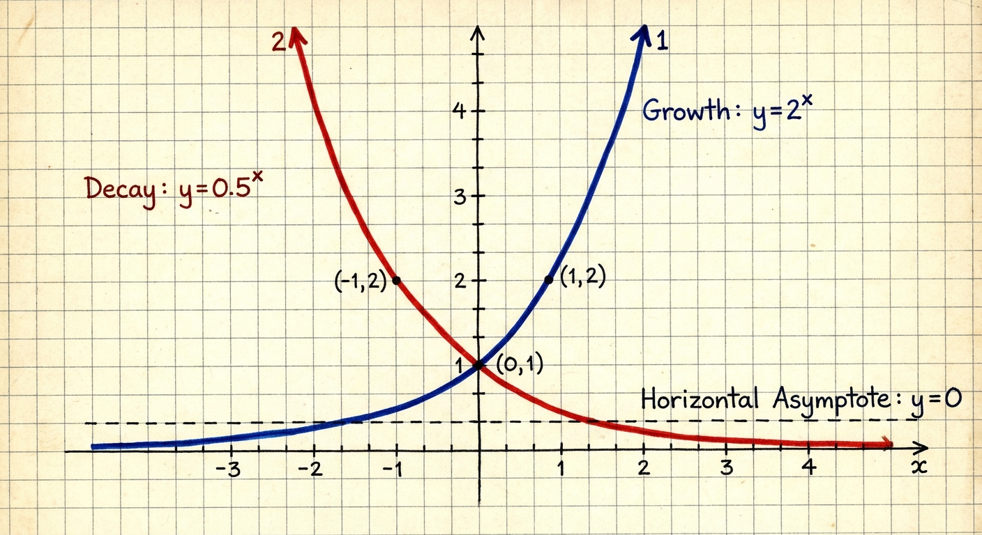
Exponential Functions and Their Graphs
An exponential function is a non-linear function where the variable acts as the exponent. These functions model phenomena where the rate of change is proportional to the current value.
Standard Form
The general form for a transformed exponential function is:
Where:
- $b$: The base (or growth/decay factor). Must be $b > 0$ and $b \neq 1$.
- $a$: Vertical stretch/compression and reflection (if $a < 0$).
- $h$: Horizontal shift.
- $k$: Vertical shift and location of the horizontal asymptote.
Key Graphing Properties
- Horizontal Asymptote: The graph approaches the line $y = k$ as $x \to -\infty$ (for growth) or $x \to \infty$ (for decay).
- Limit Notation: $ \lim_{x \to -\infty} f(x) = k $ (assuming growth).
- Y-Intercept: To find the $y$-intercept, evaluate $f(0)$. For an untransformed function $f(x) = a \cdot b^x$, the intercept is $(0, a)$.
- Domain and Range:
- Domain: $(-\infty, \infty)$
- Range: $(k, \infty)$ if $a > 0$, or $(-\infty, k)$ if $a < 0$.
- Concavity: Exponential functions of the form $f(x) = a \cdot b^x$ (where $a > 0$) are always concave up. The rate of change is constantly increasing (growth) or becoming less negative (decay).
Exponential Growth and Decay Models
The behavior of the function depends entirely on the base $b$ and the scalar $a$.
Identifying Growth vs. Decay
Assuming $a > 0$:
- Exponential Growth: Occurs when $b > 1$.
- As $x$ increases, $f(x)$ increases rapidly.
- Rate of change is positive and increasing.
- Exponential Decay: Occurs when $0 < b < 1$.
- As $x$ increases, $f(x)$ decreases toward the horizontal asymptote.
- Rate of change is negative and increasing (becoming closer to 0).
Calculating Growth/Decay Rates
In real-world problems, specific bases are often derived from a percentage rate $r$.
- If growing by 5%: $r = 0.05$, so base $b = 1.05$.
- If decaying by 12%: $r = -0.12$, so base $b = 1 - 0.12 = 0.88$.
Worked Example: Bacteria Growth
Scenario: A culture of bacteria starts with 100 cells and doubles every 3 hours.
Step 1: Identify the model structure.
We can use $N(t) = N_0 \cdot b^{(t/p)}$, where $p$ is the period.
Step 2: Plug in values.
$N_0 = 100$
Doubling implies a base of 2 occurring every 3 units of time.
Step 3: Convert to standard form (optional).
This implies an approximate 26% hourly growth rate.
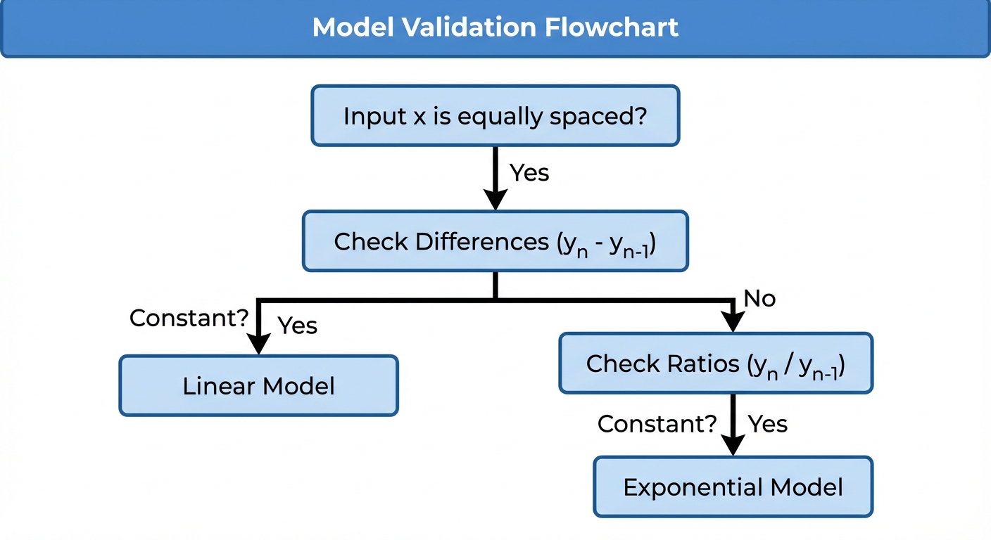
Competing Function Model Validation
A major component of AP Precalculus Unit 2 is determining whether a dataset is best modeled by a Linear or an Exponential function based on input-output patterns.
The Validation Test
If the input values ($x$) are equally spaced (e.g., $\Delta x$ is constant), analyze the output values ($y$):
Check for Linear (Arithmetic Pattern)
- Calculate the first differences between consecutive outputs.
- If the differences are constant (or approximately constant), the data is Linear.
Check for Exponential (Geometric Pattern)
- Calculate the ratios between consecutive outputs.
- If the ratios are constant (or approximately constant), the data is Exponential.
Comparison Table
| Input $x$ | Linear Output $f(x)$ | $\Delta y$ (Add) | Exponential Output $g(x)$ | Ratio $yn/y{n-1}$ (Mult) |
|---|---|---|---|---|
| 0 | 2 | - | 2 | - |
| 1 | 5 | +3 | 6 | x 3 |
| 2 | 8 | +3 | 18 | x 3 |
| 3 | 11 | +3 | 54 | x 3 |
Visual Validation (Residuals)
While calculation is preferred, you can also determine the model by plotting variables:
- Linear: A plot of $(x, y)$ yields a straight line.
- Exponential: A plot of $(x, \ln(y))$ often yields a straight line (Semi-log plot). Note: This transforms the exponential equation $y=ab^x$ into the linear form $\ln(y) = \ln(a) + x\ln(b)$.
Common Mistakes & Pitfalls
Confusing Negative Exponents with Negative Outputs
- Mistake: Thinking $2^{-3}$ is a negative number.
- Correction: $2^{-3} = \frac{1}{2^3} = \frac{1}{8}$. Exponential functions of the form $b^x$ are always positive, even with negative inputs.
Misidentifying Rates vs. Factors
- Mistake: Thinking a "15% growth rate" means $b = 0.15$.
- Correction: The rate is $r = 0.15$, so the factor (base) is $1 + r = 1.15$. $b=0.15$ would imply an 85% decay!
The Concavity Confusion
- Mistake: Assuming that because an exponential decay graph is "going down," it is concave down.
- Correction: Both standard exponential growth and decay graphs (where coefficient $a > 0$) curve upward like a cup. They are concave up. Decay decreases at a decreasing rate.
Ignoring the Asymptote in Transformations
- Mistake: Assuming the Range is always $(0, \infty)$.
- Correction: If the function is shifted vertically ($+k$), the horizontal asymptote shifts to $y=k$, making the range $(k, \infty)$.