AP Calculus BC Unit 1 (Limits and Continuity): Comprehensive Study Notes

The Big Idea of a Limit

A limit describes what value a function’s output is approaching as the input gets close to some number. The crucial word is “approaching”: a limit is about the behavior near a point, not necessarily the value at the point.

In precalculus, you often plug a number into a function to get an exact output. Calculus begins by asking a different question: what happens to the output when the input gets very close to a certain value? That’s powerful because many important situations involve values you can’t (or don’t want to) plug in directly, like a function with a hole, a jump, or an expression that becomes

$\frac{0}{0}$

Limit notation and what it means

The core notation is:

$\lim_{x \to a} f(x) = L$

Read this as: as the input approaches the number, the output approaches the limit value.

This statement does not require that the function value at the point exists, or that it equals the limit, or even that the function is defined at that input. It only requires that when the input is close to the target (on both sides), the outputs get close to the same number.

One-sided limits

Sometimes the behavior differs depending on whether you approach from the left or the right. Then you use one-sided limits.

Left-hand limit:

$\lim_{x \to a^-} f(x)$

Right-hand limit:

$\lim_{x \to a^+} f(x)$

A two-sided limit exists exactly when both one-sided limits exist and are equal.

Why limits matter (the calculus payoff)

Limits are the foundation for two central ideas you’ll soon study.

• Derivatives (instantaneous rate of change) come from limits of average rates of change.
• Integrals (accumulated change and area) come from limits of sums.

Continuity, derivatives, and many theorems in calculus are built on limits, so Unit 1 is really about learning the language and logic that the rest of the course uses.

Notation reference (common on AP questions)

You’ll commonly see these ideas tested:

• Two-sided limit: approach the input from both sides.

$\lim_{x \to a} f(x)$

• Left-hand limit: approach from values less than the target.

$\lim_{x \to a^-} f(x)$

• Right-hand limit: approach from values greater than the target.

$\lim_{x \to a^+} f(x)$

• Infinite limit: outputs grow without bound near the input.

$\lim_{x \to a} f(x) = \infty$

• Limit at infinity: end behavior as inputs increase without bound.

$\lim_{x \to \infty} f(x) = L$

Exam Focus

• Typical question patterns:
  • Given a graph (or piecewise formula), find the two-sided limit, one-sided limits, and/or the function value.
  • Decide whether a limit exists and justify using one-sided limits.
  • Interpret a limit statement in context (what it says about function behavior).
• Common mistakes:
  • Treating the limit as automatically equal to the function’s value.
  • Forgetting that a two-sided limit requires both sides to approach the same value.
  • Confusing “approaches infinity” with “equals infinity” (infinity is not a finite output value).

Estimating Limits from Graphs, Tables, and Context

A major skill in Unit 1 is reading limits from representations, especially graphs and tables. On the AP exam, you’re often given a graph or a table precisely because the function rule is unknown or complicated, so you must reason from evidence.

Ways to estimate a limit

There are a few standard approaches you should be comfortable switching between:

• Look on a graph to see what value the function is approaching.
• Estimate from a table by sampling inputs close to the target from both sides.
• Use context (real-world interpretation) to describe a trend.

From a graph: what to look for

To estimate a two-sided limit from a graph, track where the outputs head as the input gets close to the target.

Key idea: you’re “zooming in” near the target from both sides.

• If both sides head toward the same height, that height is the limit.
• If left and right head to different heights, the limit does not exist.
• If the graph shoots upward or downward without bound near the target, you may have an infinite limit.

A classic graph detail is a hole (an open circle). A hole often indicates the function is not defined there (or is defined differently), but the limit can still exist.

From a table: how to do it carefully

Tables are trickier because you’re seeing discrete samples. The best practice is to approach the target from the left using values slightly less than the target, and from the right using values slightly greater than the target, then compare outputs.

Be careful: rounding can hide differences, and some functions approach very slowly. AP questions usually make the pattern clear enough if you use both sides.

Limits in context (real-world interpretation)

Limits are often used to describe what happens “as time approaches a moment” or “as the input approaches a threshold.” For example, the temperature of an object might settle toward room temperature as time gets large, or the speed of a car might approach a value even if measurements are noisy.

In these contexts, a limit is a statement about trend, not necessarily a value actually attained at a specific instant.

Worked example 1 (graph-based reasoning)

Suppose a graph shows:

• approaching from the left, the curve approaches a height of 5,
• approaching from the right, the curve also approaches a height of 5,
• there is an open circle at that height, and a filled dot at height 1.

Then the limit is 5, but the function value at the point is 1. This is a perfect illustration that a limit and a function value can differ.

Worked example 2 (table-based estimation)

A table gives values near 3:

From the left, values approach about 7. From the right, values also approach about 7. So you estimate:

$\lim_{x \to 3} f(x) = 7$

Notice the table does not tell you the exact value at 3 unless it explicitly includes that input.

Exam Focus

• Typical question patterns:
  • “Estimate the limit from the table/graph. Does it appear to exist?”
  • “Given the graph, find one-sided limits and determine continuity at the target input.”
  • “Given values of a function near a point, choose a statement that must be true.”
• Common mistakes:
  • Using only one side of the table and assuming the two-sided limit exists.
  • Reading the filled dot as the limit instead of focusing on the approaching behavior.
  • Confusing a steep graph with “limit does not exist” when it actually approaches a finite value.

Evaluating Limits Analytically (Algebra and Function Properties)

When you have a formula for a function, you often evaluate limits using algebra and known limit properties. The core strategy is:
1) try direct substitution, 2) if substitution fails (often due to an indeterminate form), simplify the expression, 3) re-evaluate the simplified limit.

Direct substitution and when it works

If a function is well-behaved near the target input (for example, a polynomial), then the limit equals the function value you get by plugging in. In particular, to find the limit of a simple polynomial, you can plug in the number being approached because polynomials are continuous everywhere.

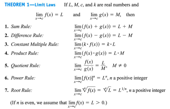
Limit laws (algebraic properties)

Limit laws justify why algebraic simplification works. If the limits of two functions exist, then the limit of their sum is the sum of their limits, the limit of their product is the product of their limits, and the limit of their quotient is the quotient of their limits (as long as the denominator limit is not zero).

Here is a commonly used summary chart of algebraic properties:

The indeterminate form

If direct substitution yields

$\frac{0}{0}$

that does not mean the limit is 0 or “automatically undefined.” It means the expression is indeterminate, and you need to rewrite it.

Typical tools:

• factoring and canceling a common factor
• rationalizing (using conjugates)
• combining fractions
• using special trig limits (covered in the trig section)

A key idea here is removable discontinuity: if a factor cancels, the simplified expression describes the behavior near the point, even if the original function had a hole at that input.

Algebraic manipulation and removable discontinuities

A common move is to factor the numerator and denominator, then cancel any common factors (which correspond to removable discontinuities). This is especially useful when substitution makes the denominator equal to 0.

For example:

$\frac{(x+3)(x+2)}{(x+3)(x-3)}$

The factor

$x+3$

can be removed (for inputs where it is not zero), which indicates a removable discontinuity at the input that makes that factor zero.

Important accuracy note: “removing a discontinuity” typically means simplifying the formula to remove the hole-causing factor and, if you want the function itself to be continuous, redefining the function’s value at the missing input to equal the limit.

Example 1: factoring and canceling

Evaluate:

$\lim_{x \to 2} \frac{x^2-4}{x-2}$

Direct substitution gives an indeterminate form, so factor:

$x^2-4=(x-2)(x+2)$

For inputs not equal to 2, the expression simplifies to

$x+2$

So the limit is

$\lim_{x \to 2} (x+2)=4$

Conceptually, the original function behaves like the line near 2, except it has a hole at 2.

Example 2: rationalizing a radical expression

Evaluate:

$\lim_{x \to 0} \frac{\sqrt{1+x}-1}{x}$

Multiply by the conjugate:

$\frac{\sqrt{1+x}-1}{x} \cdot \frac{\sqrt{1+x}+1}{\sqrt{1+x}+1}=\frac{(1+x)-1}{x(\sqrt{1+x}+1)}$

Simplify:

$\frac{(1+x)-1}{x(\sqrt{1+x}+1)}=\frac{1}{\sqrt{1+x}+1}$

Now substitute:

$\lim_{x \to 0} \frac{1}{\sqrt{1+x}+1}=\frac{1}{2}$

Piecewise-defined functions (limits and values can differ)

AP loves piecewise functions because they test whether you understand “approach” rather than “plug in.” To find a two-sided limit at a boundary input, you must compute the left-hand limit using the rule valid on the left side and compute the right-hand limit using the rule valid on the right side, then compare.

Even if the function value at the boundary is defined by a separate rule, that function value alone does not determine the limit.

Exam Focus

• Typical question patterns:
  • Evaluate limits that give an indeterminate form using factoring, canceling, and algebra.
  • For a piecewise function, compute the left-hand and right-hand limits and decide if the two-sided limit exists.
  • Identify which limit laws justify a step in simplification.
• Common mistakes:
  • Canceling terms incorrectly (for example, canceling across addition).
  • Declaring “undefined” immediately when seeing an indeterminate form instead of simplifying.
  • Using the formula piece that includes the boundary input to compute a limit, rather than using the behavior on each side.

Special Trigonometric Limits and the Squeeze Theorem

Trigonometric limits show up frequently because trig functions model periodic phenomena, and because derivatives of trig functions rely on a few foundational limits.

The foundational trig limits (radians)

A central result (used later to derive derivatives of sine and cosine) is:

$\lim_{x \to 0} \frac{\sin x}{x}=1$

This is true when angles are measured in radians (AP Calculus assumes radians unless explicitly stated otherwise).

Closely related limits you’ll see in problems include:

$\lim_{x \to 0} \frac{1-\cos x}{x}=0$

and the equivalent sign-swapped version:

$\lim_{x \to 0} \frac{\cos x-1}{x}=0$

A very common and more useful form is:

$\lim_{x \to 0} \frac{1-\cos x}{x^2}=\frac{1}{2}$

Two additional trig limit patterns that are frequently tested are:

$\lim_{x \to 0} \frac{\sin(ax)}{x}=a$

and

$\lim_{x \to 0} \frac{\sin(ax)}{\sin(bx)}=\frac{a}{b}$

How to use trig limits (pattern matching through algebra)

When you see something like sine of a multiple of the variable, your goal is to build the pattern “sine over its angle.” For example, you often multiply and divide by the constant so that the denominator matches the inside of the sine.

Worked example 1: using the sine-over-angle limit

Evaluate:

$\lim_{x \to 0} \frac{\sin(3x)}{x}$

Rewrite:

$\frac{\sin(3x)}{x}=3\cdot\frac{\sin(3x)}{3x}$

Then the limit is:

$\lim_{x \to 0} 3\cdot\frac{\sin(3x)}{3x}=3$

Worked example 2: using a conjugate with trig

Evaluate:

$\lim_{x \to 0} \frac{1-\cos x}{x^2}$

Multiply by the conjugate:

$\frac{1-\cos x}{x^2}\cdot\frac{1+\cos x}{1+\cos x}=\frac{1-\cos^2 x}{x^2(1+\cos x)}$

Use the identity:

$1-\cos^2 x=\sin^2 x$

So the expression becomes:

$\frac{\sin^2 x}{x^2(1+\cos x)}=\left(\frac{\sin x}{x}\right)^2\cdot\frac{1}{1+\cos x}$

Now take limits:

$\lim_{x \to 0} \left(\frac{\sin x}{x}\right)^2=1$

and

$\lim_{x \to 0} (1+\cos x)=2$

So:

$\lim_{x \to 0} \frac{1-\cos x}{x^2}=\frac{1}{2}$

The Squeeze Theorem

The Squeeze Theorem is used when a function is hard to analyze directly but can be trapped between two simpler functions that share the same limit.

If for all inputs near the target (except possibly at the target itself) you have:

$g(x) \le f(x) \le h(x)$

and

$\lim_{x \to a} g(x)=L$

and

$\lim_{x \to a} h(x)=L$

then:

$\lim_{x \to a} f(x)=L$

Worked example 3: a classic squeeze

Evaluate:

$\lim_{x \to 0} x^2\sin\left(\frac{1}{x}\right)$

Even though the sine term oscillates, you always know:

$-1 \le \sin\left(\frac{1}{x}\right) \le 1$

Multiply all parts by the nonnegative quantity:

$x^2$

to get:

$-x^2 \le x^2\sin\left(\frac{1}{x}\right) \le x^2$

Both bounding functions approach 0 as the input approaches 0, so the squeezed function must also approach 0.

Exam Focus

• Typical question patterns:
  • Evaluate trig limits by rewriting to match the sine-over-angle form or using conjugates.
  • Use and recognize the patterns involving constants (like the limits for %%LATEX45%% and %%LATEX46%%).
  • Identify when the Squeeze Theorem applies and use it to find a limit.
  • Explain (briefly) why radians are required for standard trig limits.
• Common mistakes:
  • Forgetting to convert to a sine-over-angle form and trying to substitute too early.
  • Misapplying squeeze without showing both bounding functions approach the same limit.
  • Using degrees in trig limits.

Limits Involving Infinity: Vertical Asymptotes and End Behavior

Some limits do not approach a finite number. Instead, the function may grow without bound near a point (vertical asymptote behavior) or settle toward a value as inputs become very large (horizontal asymptote or end behavior).

Infinite limits (approaching a vertical asymptote)

An infinite limit describes outputs that grow without bound as the input approaches a value.

For example:

$\lim_{x \to a} f(x)=\infty$

means: as the input gets close to the target, the output grows larger than any fixed number.

Similarly:

$\lim_{x \to a} f(x)=-\infty$

means the outputs decrease without bound.

Often this happens when a denominator approaches 0 while the numerator stays nonzero.

One-sided infinite limits matter

A vertical asymptote often has different behavior on each side, so one-sided limits are essential.

Example 1: detecting a vertical asymptote

Evaluate:

$\lim_{x \to 2^-} \frac{1}{x-2}$

and

$\lim_{x \to 2^+} \frac{1}{x-2}$

Approaching from the left makes the denominator a small negative number, so the fraction becomes a large negative number. Approaching from the right makes the denominator a small positive number, so the fraction becomes a large positive number:

$\lim_{x \to 2^-} \frac{1}{x-2}=-\infty$

$\lim_{x \to 2^+} \frac{1}{x-2}=\infty$

So there is a vertical asymptote at 2. A vertical asymptote is a vertical line where the function is undefined or becomes unbounded, so the graph has no point on that line.

Limits at infinity (end behavior) and horizontal asymptotes

A limit at infinity describes what happens as inputs grow without bound:

$\lim_{x \to \infty} f(x)=L$

or as inputs decrease without bound:

$\lim_{x \to -\infty} f(x)=L$

If the limit equals a finite number, then the line at that output value is a horizontal asymptote in that direction.

Important nuance: a horizontal asymptote can be crossed. It describes end behavior, not a barrier.

Rational functions at infinity (degree reasoning)

Let

$f(x)=\frac{P(x)}{Q(x)}$

where the numerator and denominator are polynomials.

• If degree of the numerator is less than degree of the denominator, then the limit at infinity is 0 and the horizontal asymptote is the line “output equals 0.”
• If degrees are equal, the limit is the ratio of leading coefficients.
• If degree of the numerator is greater than degree of the denominator, then the function does not approach a finite horizontal asymptote. In many AP-style problems, the limit as inputs go to infinity will be unbounded (often described as “the limit is infinity” in the sense of diverging), so there is no horizontal asymptote.

These are the same horizontal asymptote rules often summarized as:

• highest power in the numerator: the limit at infinity is unbounded, so no horizontal asymptote
• highest power in the denominator: the limit at infinity is 0, so horizontal asymptote is output equals 0
• same highest power: limit is leading coefficient ratio

Worked example 2: degrees and leading coefficients

Evaluate:

$\lim_{x \to \infty} \frac{3x^2-5}{2x^2+7x+1}$

Degrees match, so the limit is the ratio of leading coefficients:

$\lim_{x \to \infty} \frac{3x^2-5}{2x^2+7x+1}=\frac{3}{2}$

So the horizontal asymptote (as inputs go to positive infinity, and also to negative infinity for this example) is the line at output value

$\frac{3}{2}$

Worked example 3: tending to 0

Evaluate:

$\lim_{x \to \infty} \frac{5x-1}{x^2+4}$

The denominator has higher degree, so the limit is:

$\lim_{x \to \infty} \frac{5x-1}{x^2+4}=0$

Exam Focus

• Typical question patterns:
  • Compute one-sided limits that lead to unbounded behavior and interpret vertical asymptotes.
  • Evaluate limits at infinity for rational functions using degree comparisons.
  • Match a limit statement to a graph description (end behavior or asymptote behavior).
• Common mistakes:
  • Saying the limit “equals infinity” as if infinity were a number you reach (treat it as unbounded growth).
  • Forgetting one-sided analysis near vertical asymptotes.
  • Using degree rules incorrectly (for equal degrees, use leading coefficients).

Continuity: What It Means and How to Check It

Continuity is the idea that a function has no breaks in its graph at a point or over an interval. In calculus, continuity is essential because many theorems and later techniques rely on it.

Continuity at a point (formal conditions)

A function is continuous at a target input if all three of these are true:
1) the function value exists,
2) the limit exists,
3) the limit equals the function value.

This definition forces you to separate three ideas: the function’s actual value, the approaching behavior from both sides, and whether those match.

Continuity over an interval

A function is continuous on an interval if it is continuous at every point of that interval. On a closed interval, continuity at endpoints is checked with the appropriate one-sided limit (approaching from within the interval).

Types of discontinuities (how graphs “break”)

When continuity fails, it often fails in recognizable ways.

Removable discontinuity (a hole)

A removable discontinuity occurs when the limit exists but the function value is missing or does not match the limit. Graphically it looks like a hole. It is “removable” because you can remove the discontinuity by filling the hole at the limit value (equivalently, by redefining the function’s value at that input to equal the limit).

Jump discontinuity

A jump discontinuity occurs when the left-hand and right-hand limits both exist and are finite, but they do not match. The graph breaks and “starts” at a different height.

Essential/infinite discontinuity (vertical asymptote)

An essential (often called infinite) discontinuity occurs when the function has a vertical asymptote and becomes unbounded near the input.

Removing discontinuities (what you actually do)

In practice, removable discontinuities are frequently handled by factoring out a common factor in a rational expression (a common root shared by numerator and denominator). After simplification, you can define the function at the missing input so that its value matches the limit, making the function continuous there.

Example 1: making a function continuous by choosing a value

Suppose the function is defined by:

$f(x)=\frac{x^2-1}{x-1} \text{ for inputs not equal to 1}$

and

$f(1)=c$

To make the function continuous at 1, set the function value equal to the limit:

$c=\lim_{x \to 1} \frac{x^2-1}{x-1}$

Factor:

$\frac{x^2-1}{x-1}=\frac{(x-1)(x+1)}{x-1}=x+1$

So:

$c=\lim_{x \to 1} (x+1)=2$

Example 2: checking continuity at a point

Let

$g(x)=x+2 \text{ for inputs less than 0}$

and

$g(x)=x^2 \text{ for inputs greater than or equal to 0}$

Check continuity at 0. The left-hand limit is 2 and the right-hand limit is 0, so the two-sided limit does not exist and the function is not continuous there (jump discontinuity). Even though the function value at 0 exists, continuity requires the limit to exist and match.

Why continuity matters in practice

Continuity is the mathematical version of “no sudden breaks.” In modeling, a position function that jumps instantly is physically unrealistic, and a temperature function that jumps might indicate a phase change or measurement issues. In calculus techniques later, continuity often allows direct substitution, supports theorems, and guarantees solutions exist.

Exam Focus

• Typical question patterns:
  • Determine where a function is continuous/discontinuous from a graph or formula.
  • Classify discontinuities (removable, jump, infinite) using limits.
  • Find a constant parameter so that a piecewise function is continuous at a point.
• Common mistakes:
  • Thinking “the limit exists” automatically means “the function is continuous” (you also need the function value and equality).
  • Classifying a discontinuity without checking one-sided limits.
  • At endpoints, incorrectly using two-sided limits instead of the appropriate one-sided limit.

The Intermediate Value Theorem (IVT) and What Continuity Guarantees

The Intermediate Value Theorem is a main payoff of continuity: if a function is continuous, it cannot skip over output values.

Statement of the Intermediate Value Theorem

If a function is continuous on a closed interval from a to b, and a number lies between the outputs at the endpoints, then there exists at least one input in the interval where the function equals that number.

Formally:

$\text{If } f \text{ is continuous on } [a,b] \text{ and } N \text{ is between } f(a) \text{ and } f(b), \text{ then } \exists c \in [a,b] \text{ such that } f(c)=N$

Why IVT matters

IVT is a guarantee of existence. It does not tell you exactly where the solution is, and it does not tell you how many solutions there are.

How to use IVT (the practical recipe)

To use IVT to prove an equation has a solution on an interval:
1) define a continuous function whose zeros correspond to the equation,
2) verify continuity on the entire closed interval,
3) compute endpoint values,
4) show the target value is between them (often by showing opposite signs when the target is 0).

Worked example 1: proving a root exists

Show that the equation

$x^3+x-1=0$

has a solution in the interval from 0 to 1.

Let

$f(x)=x^3+x-1$

This is a polynomial, so it is continuous. Compute:

$f(0)=-1$

$f(1)=1$

Since 0 lies between -1 and 1, IVT guarantees a solution in the open interval.

Worked example 2: what IVT does NOT guarantee

If a continuous function has values -3 at one endpoint and 4 at the other, IVT guarantees at least one point where the function equals 0 somewhere between. But IVT does not guarantee uniqueness, monotonicity, or that you can find an exact value without other methods.

A common misconception: discontinuous functions can “skip” values

A function with a jump discontinuity can leap from one output value to another without ever taking intermediate values. That is exactly why the continuity condition is essential.

Exam Focus

• Typical question patterns:
  • Use IVT to justify that an equation has a root on an interval.
  • Given a function (often polynomial or trig), show there exists a solution to an equation of the form function equals a constant on an interval.
  • Explain why IVT applies (explicitly mention continuity on the closed interval and the “between values” condition).
• Common mistakes:
  • Forgetting to state (or verify) continuity on the entire closed interval.
  • Claiming IVT finds the solution, rather than guarantees existence.
  • Using IVT when the endpoint outputs are not on opposite sides of the target value.

Putting It Together: Strategy, Justification, and Clear Communication

Unit 1 is not just about getting answers; it’s about choosing valid methods and justifying conclusions. On AP free-response especially, you’re expected to write mathematically correct reasoning.

A reliable limit-solving decision process

When you’re asked to evaluate a limit from a formula, a strong approach is:
1) Try substitution. If you get a finite number, you’re usually done.
2) If you get an indeterminate form, simplify (factor/cancel, rationalize, combine terms, or use trig identities).
3) If values blow up, consider infinite limits and one-sided behavior.
4) If it’s oscillatory but bounded, consider the Squeeze Theorem.

Justifying “limit exists” vs “limit does not exist”

A common AP prompt is: “Does the limit exist? Explain.” Your explanation should match the reason.

• If left and right limits are different, explicitly state both values.
• If the function is unbounded, state it approaches infinity or negative infinity (often one-sided).
• If the function approaches a finite value from both sides, state that value.

A model justification looks like this: the left-hand limit equals one number and the right-hand limit equals a different number, so the two-sided limit does not exist because the one-sided limits are not equal.

Continuity arguments: the 3-condition checklist (used naturally)

When continuity is tested, strong written solutions address: is the function defined at the input, does the two-sided limit exist, and does the limit match the function value?

If you’re solving for a parameter to make a function continuous, the key move is setting the value equal to the limit and then solving for the parameter.

Common traps across the unit

• Confusing a hole with a non-existent limit (holes often still have a limit).
• Treating infinity like a number (it describes unbounded growth).
• Forgetting the two-sided limit requirement (both sides must agree).
• Using the wrong tool (for example, applying degree rules to something that is not a rational function).

A final connection forward

As you move into derivatives, you’ll repeatedly rely on Unit 1 ideas: derivatives use limits of difference quotients, differentiability implies continuity (one-way), and “local” graph behavior near points is best discussed using limits.

Exam Focus

• Typical question patterns:
  • “Evaluate the limit and show work” where scoring depends on a correct method (factoring, conjugates, trig limits).
  • “Does the limit exist?” requiring a one-sided limit argument or a statement about unbounded behavior.
  • “Find a parameter so that a function is continuous at the target input,” which requires setting the function value equal to a limit.
• Common mistakes:
  • Providing an answer without justification when the question explicitly asks for reasoning.
  • Mixing up the roles of function value, two-sided limit, and one-sided limits in continuity questions.
  • Doing correct algebra but evaluating the wrong limit (approaching the wrong input or ignoring one-sided directions).