Mastering Continuity: Concepts, Theorems, and Analysis
Defining Continuity at a Point
In calculus, the concept of continuity formalizes the intuitive idea of drawing a curve without lifting your pencil from the paper. While that visual definition helps, AP Calculus BC requires a rigorous, three-part algebraic definition to prove continuity at a specific $x$-value.
The Three-Part Definition
For a function $f(x)$ to be continuous at a point $x = c$, three specific conditions—often called the continuity test—must be met:
- $f(c)$ is defined: The function must have a specific value at $x = c$ (it is part of the domain).
- $\lim{x \to c} f(x)$ exists: The left-hand limit and the right-hand limit must be equal to a finite number.
- $\lim_{x \to c} f(x) = f(c)$: The limit as $x$ approaches $c$ must equal the actual function value at $c$.
If any of these three conditions fails, the function is discontinuous at $x = c$.
Types of Discontinuities
Discontinuities occur when the continuity test fails. On the AP exam, you must be able to identify these graphically and justify them using limits.
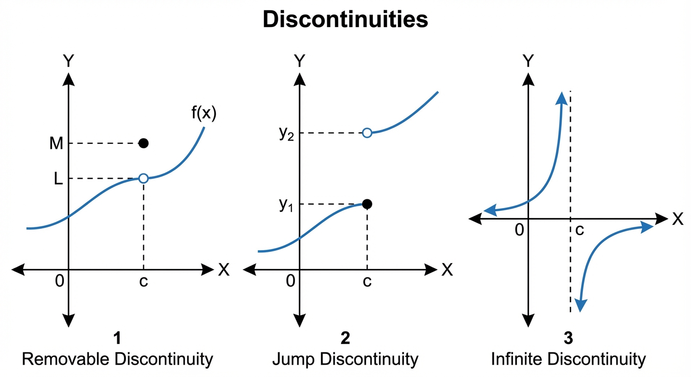
1. Removable Discontinuity (Hole)
This occurs when the limit exists (Condition 2 passes), but the function fails Condition 3. This means there is a "hole" in the graph.
- Algebraic Clue: In a rational function, common factors in the numerator and denominator often indicate a removable discontinuity.
- Example:
There is a hole at $x=1$ because the limit exists (it equals 2), but $f(1)$ is undefined.
2. Jump Discontinuity
This occur when the limit does not exist because the left-hand limit and right-hand limit are finite but different.
- Algebraic Clue: Often seen in piecewise functions or step functions (like the floor function).
- Condition:
3. Infinite Discontinuity (Vertical Asymptote)
This occurs when the limit as $x$ approaches $c$ is positive or negative infinity.
- Algebraic Clue: In a rational function, a denominator is zero while the numerator is non-zero.
Note: Both Jump and Infinite discontinuities are considered non-removable.
| Discontinuity Type | Limit Exists? | Function Defined? | Limit = Function? | Removable? |
|---|---|---|---|---|
| Hole | Yes | Maybe | No | Yes |
| Jump | No | Maybe | N/A | No |
| Infinite | No | No | N/A | No |
Removing Discontinuities
Removing a discontinuity refers to re-defining (or defining) the function at a specific point so that it becomes continuous there. This is only possible for Removable Discontinuities.
The Concept of the Extended Function
If $f(x)$ has a removable discontinuity at $x=c$ and the limit is $L$, we can define a new continuous function $g(x)$:
Worked Example
Problem: Let . Find the value $k$ that makes the function continuous at $x=5$ if we define $f(5) = k$.
Solution:
- Check the limit: Plug in $x=5$ to see the form $\frac{25-15-10}{5-5} = \frac{0}{0}$. This suggests a limit likely exists.
- Factor and Simplify:
- Evaluate:
- Conclusion: Since the limit is 7, we must define $f(5) = 7$ to make the function continuous. Therefore, $k=7$.
Continuity over an Interval
While point-continuity focuses on a single $x$-value, interval continuity focuses on a range.
Open Intervals $(a, b)$
A function is continuous on an open interval $(a, b)$ if it is continuous at every point inside that interval.
Key Rule: Most standard functions—polynomials, rational functions, trigonometric functions, exponentials, and logarithms—are continuous everywhere in their domains.
Closed Intervals $[a, b]$
Continuity on a closed interval includes definitions for the endpoints. A function is continuous on $[a, b]$ if:
- It is continuous on the open interval $(a, b)$.
- It is right-continuous at $x = a$ (limit from the right equals $f(a)$).
- It is left-continuous at $x = b$ (limit from the left equals $f(b)$).
The Intermediate Value Theorem (IVT)
The IVT is an existence theorem. It doesn't tell you how to find a value, only that the value exists. This is a frequent topic on AP Free Response Questions (FRQs).
The Theorem Statements
If a function $f$ is continuous on the closed interval $[a, b]$, and $k$ is any number strictly between $f(a)$ and $f(b)$, then there exists at least one number $c$ in the interval $(a, b)$ such that $f(c) = k$.
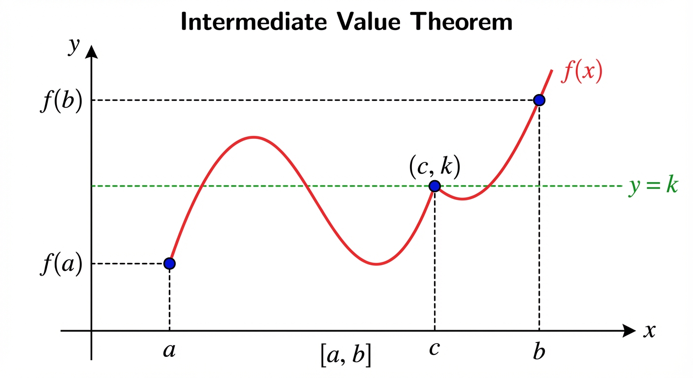
Why is this useful?
It allows us to prove that a function hits a specific target value. The most common application is proving a function has a zero (or root). If $f(a)$ is negative and $f(b)$ is positive (and $f$ is continuous), the function must cross the x-axis somewhere between $a$ and $b$.
How to Write an IVT Justification on the AP Exam
For full credit on an FRQ, you must follow this template strictly:
- State Conditions: "Since $f(x)$ is continuous on the closed interval $[a, b]$…"
- Evaluate Endpoints: "…and $f(a) = y1$ and $f(b) = y2$…"
- Establish Inequality: "…and since $k$ is between $y1$ and $y2$…"
- Conclude: "…by the Intermediate Value Theorem, there exists a value $c$ in $(a, b)$ such that $f(c) = k$."
Example Application:
Show that $f(x) = x^3 - x - 1$ has a root between $x=1$ and $x=2$.
- Continuity: $f(x)$ is a polynomial, so it is continuous on $[1, 2]$.
- Endpoints:
- Inequality: We are looking for a root ($k=0$). Since $-1 < 0 < 5$…
- Conclusion: By the IVT, there is a $c$ in $(1, 2)$ where $f(c) = 0$.
Common Mistakes & Pitfalls
- Confusing Limits with Function Values: Specifically, assuming that just because a limit exists, the function is continuous. Remember the example of the hole: limit exists, function doesn't.
- Neglecting Conditions for IVT: Students often forget to explicitly write "continuous on the closed interval $[a, b]$." Without continuity, the IVT does not apply. Just checking the endpoints is not enough.
- Mixing up "Removable" and "Non-Removable":
- Can you fix it by filling 1 single pixel? -> Removable.
- Do you have to redraw the curve? -> Non-removable.
- Endpoint Behavior: Forgetting that on a closed interval $[a, b]$, limits at the endpoints are only one-sided.