Unit 7 Study Notes: Understanding Differential Equations
Introduction to Modeling Change
Calculus is fundamentally the study of change. In previous units, you learned that the derivative, $\frac{dy}{dx}$, represents the instantaneous rate of change of a quantity. In Unit 7, we reverse this process. Instead of starting with a function and finding its derivative, we start with an equation involving a derivative—a Differential Equation—and work backward to find the original function.
What is a Differential Equation?
A differential equation (DE) is an equation that relates a function $y$, its independent variable $x$, and one or more of its derivatives (like $y'$ or $y''$).
- Goal: To find a function $y = f(x)$ that makes the equation true.
- General Solution: A family of functions containing an arbitrary constant $C$ (e.g., $y = x^2 + C$). This represents all possible curves that satisfy the rate of change.
- Particular Solution: A specific function (e.g., $y = x^2 + 5$) found by using an initial condition (a known point $(x, y)$) to solve for $C$.
Verifying Solutions
Before you learn to solve them from scratch, you must know how to check if a function is a valid solution to a differential equation.
The Method
- Differentiate: Take the derivative of the proposed solution $y$.
- Substitute: Plug $y$ and $\frac{dy}{dx}$ into the given differential equation.
- Verify: Check if the left-hand side (LHS) equals the right-hand side (RHS).
Example:
Is $y = e^{-3x}$ a solution to the differential equation $y' + 3y = 0$?
- Step 1: Find $y'$. Using the chain rule, $y' = -3e^{-3x}$.
- Step 2: Substitute into the DE.
- Step 3: Simplify.
Since $0=0$, it is a solution.
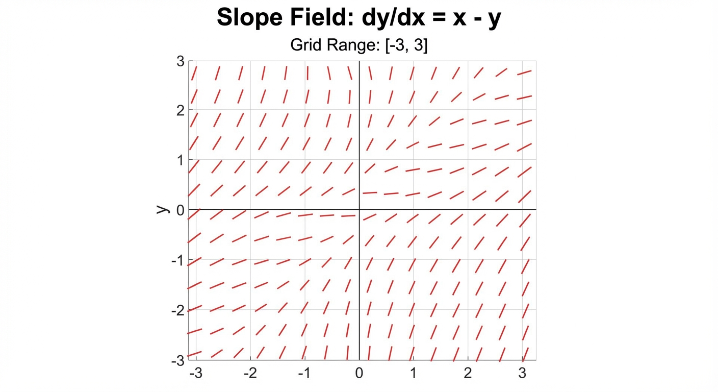
Slope Fields
Algebraic solutions aren't the only way to understand differential equations. Slope Fields provide a geometric (visual) representation of the general solution.
What is a Slope Field?
A slope field is a graph composed of many small line segments drawn at coordinate grid points. At any specific point $(x, y)$, the derivative $\frac{dy}{dx}$ gives you the slope of the tangent line at that point.
Constructing a Slope Field
To draw a slope field manually:
- Pick a point on the grid, say $(1, 2)$.
- Plug these coordinates into the differential equation to find the slope value.
- Draw a short line segment at $(1, 2)$ with that specific slope.
- Repeat for other points.
Tip: Look for patterns to save time.
- If the DE is $\frac{dy}{dx} = x$ (depends only on $x$), the slopes will be identical in every vertical column.
- If the DE is $\frac{dy}{dx} = y$ (depends only on $y$), the slopes will be identical in every horizontal row.
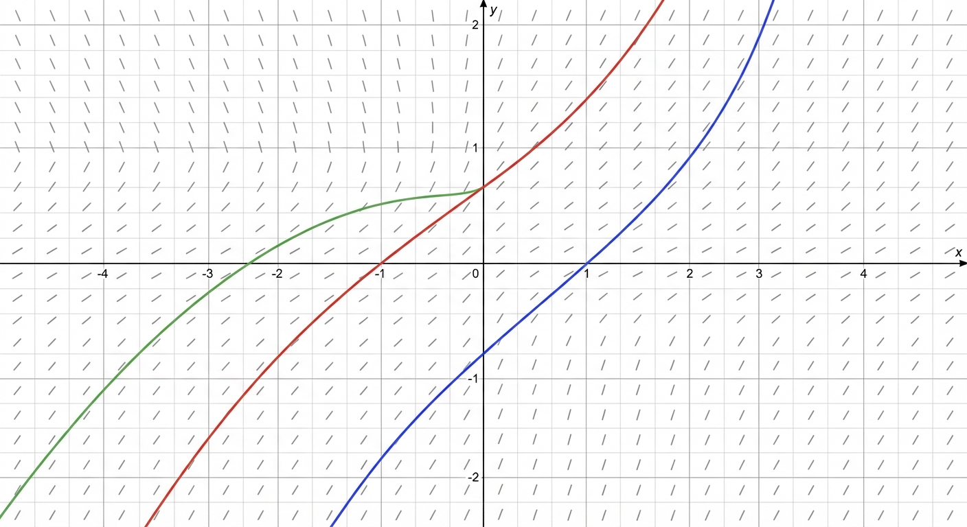
Sketching Solution Curves
The AP Exam often asks you to sketch a particular solution curve passing through a given initial point.
The Strategy: "Go with the Flow"
- Mark the Start: Plot the given initial condition point (e.g., $(0, 1)$).
- Follow the Lines: Draw a curve that moves significantly parallel to the nearby slope segments. Think of the slope segments as currents in a river; your line should flow with them.
- Boundaries: Your curve should extend to the edges of the graph unless it hits an asymptote or a place where the derivative is undefined.
Solving by Separation of Variables
This is the most critical algebraic skill in Unit 7. When given a first-order differential equation, you must rearrange it so all $y$ terms are on one side and all $x$ terms are on the other before integrating.
The SIPPY Method
A mnemonic to remember the steps for finding a particular solution is SIPPY:
- S - Separate: Multiply/divide to get $dy$ with $y$ terms on the left, and $dx$ with $x$ terms on the right.
- I - Integrate: Apply $\int$ to both sides.
- P - Plus C: Immediately add $+C$ to the $x$-side (right side).
- P - Plug In: Substitute the initial condition $(x, y)$ to solve for $C$.
- Y - Y equals: Algebraically manipulate the equation to isolate $y$.
Worked Example
Problem: Find the particular solution to $\frac{dy}{dx} = \frac{4x}{y}$ with initial condition $y(0) = 5$.
1. Separate:
multiply both sides by $y$ and by $dx$:
2. Integrate:
3. Plus C:
Do not forget this step!
4. Plug In:
Use $x=0, y=5$ to find $C$:
Update equation: $\frac{y^2}{2} = 2x^2 + \frac{25}{2}$
5. Y equals:
Isolate $y$. First, multiply by 2:
Take the square root:
Crucial Decision: Since our initial $y$ was positive ($5$), we keep the positive root.
Final Solution:
Exponential Models
A specific type of differential equation appears frequently in real-world modeling (population growth, radioactive decay).
The Law of Exponential Change
If the rate of change of a quantity $y$ is proportional to the quantity itself, we write:
Where $k$ is the constant of proportionality.
- If $k > 0$: Exponential Growth (Population, Bacteria)
- If $k < 0$: Exponential Decay (Radioactive isotopes)
The General Solution
You can solve this using Separation of Variables, but you should memorize the result:
- $y(t)$ = amount at time $t$
- $y_0$ = initial amount (at $t=0$)
Newton's Law of Cooling
Sometimes rate of change depends on the difference between the object's temperature ($T$) and the surrounding room temperature ($Ts$).
To solve this, treat $(T - T_s)$ as a single variable during separation:
- $\frac{1}{T-T_s} dT = k \, dt$
- Integrate to get $\ln|T - T_s| = kt + C$
- Exponentiate both sides to solve for $T$.
Common Mistakes & Pitfalls
The Missing "+C":
- Mistake: Forgetting to write $+C$ immediately after integrating.
- Correction: If you add $C$ at the very end, your algebra will be wrong (e.g., $e^{x+C}$ is very different from $e^x + C$).
Bad Separation Algebra:
- Mistake: If $\frac{dy}{dx} = x + y$, students often try to divide by $y$ to get $\frac{1}{y}dy = x dx$. This is illegal. You can only separate by multiplication or division.
- Note: $\frac{dy}{dx} = x+y$ cannot be solved by separation of variables.
Ignoring Absolute Values with Logarithms:
- Mistake: Integrating $\int \frac{1}{y} dy = \ln(y)$.
- Correction: The integral is $\ln|y| + C$. The absolute value matters for determining the domain and the correct branch of the solution.
Slope Field Sloppiness:
- Mistake: Drawing a solution curve that crosses through a region where the slope is undefined, or crossing over its own asymptote.
- Correction: Solution curves are continuous functions. They cannot jump over asymptotes.
Picking the Wrong Root:
- Mistake: Leaving the answer as $y = \pm\sqrt{…}$ or arbitrarily picking positive.
- Correction: Check your initial condition. If $y(0) = -3$, your solution must involve the negative root ($y = -\sqrt{…}$).