AP Calculus AB Unit 1 Study Guide: Limits, Continuity, and Core Strategies

Change in a Function and Average Rate of Change

Calculus starts with a simple idea: you want to describe how quantities change. Before you ever take a limit, you should be comfortable describing change over an interval.

Change and average rate of change

If a function models some quantity (height, cost, position, temperature), then change compares the output values between two inputs.

The change in the function from %%LATEX0%% to %%LATEX1%% is

$f(b)-f(a)$

The average rate of change over $[a,b]$ tells you “change in output per change in input”:

$\text{Average rate of change on }[a,b]=\frac{f(b)-f(a)}{b-a}$

This matters because average rate of change is the slope of the secant line through the points %%LATEX5%% and %%LATEX6%%. Later, calculus asks what happens to this average rate of change as the interval shrinks until it becomes “instantaneous.” That idea is built from limits.

Interpreting units and meaning

Average rate of change is not just a computation; it has meaning.

If %%LATEX7%% is in dollars and %%LATEX8%% is in months, then average rate of change has units “dollars per month.” A positive rate means the function is increasing on that interval, and a negative rate means decreasing.

Worked example: average rate of change

Suppose

$f(x)=x^2$

Find the average rate of change on $[2,5]$.

Compute the function values: %%LATEX11%% and %%LATEX12%%. Then

$\frac{f(5)-f(2)}{5-2}=\frac{25-4}{3}=\frac{21}{3}=7$

Interpretation: over $2 \le x \le 5$, the function increases by 7 units of output for each 1 unit of input, on average.

Connecting to “zooming in”

If you compute average rates of change on smaller and smaller intervals around a point, you often see them approach a single value. That “approach” is exactly what limits formalize.

Exam Focus

Typical question patterns:

• Compute and interpret average rate of change on an interval (often with units or context).
• Compare average rates of change on different intervals and relate to increasing/decreasing behavior.

Common mistakes:

• Swapping %%LATEX15%% and %%LATEX16%% inconsistently (leading to sign errors).
• Forgetting the denominator is %%LATEX17%% (change in input), not just %%LATEX18%%.

What a Limit Is (and What It Is Not)

Limits are the value that a function approaches as the variable gets nearer to a particular value. The key mindset is that we don’t really care what’s happening at the point; we care about what’s happening around the point.

The core idea: approaching vs. arriving

When you write

$\lim_{x\to a} f(x)=L$

you are saying you can make %%LATEX20%% as close to %%LATEX21%% as you want by taking %%LATEX22%% sufficiently close to %%LATEX23%%, without requiring $x=a$.

This is why limits can exist even if:

• $f(a)$ is undefined (a hole).
• $f(a)$ exists but is not equal to the limit.
• the graph has a break at $a$.

A key misconception is thinking %%LATEX28%% means “plug in %%LATEX29%%.” Plugging in is only one strategy, and it works only when the function is well-behaved (continuous) at $a$.

One-sided limits

Sometimes behavior depends on approaching from the left versus the right.

Left-hand limit:

$\lim_{x\to a^-} f(x)=L$

Right-hand limit:

$\lim_{x\to a^+} f(x)=R$

The two-sided limit exists precisely when both one-sided limits exist and match:

$\lim_{x\to a} f(x) \text{ exists if and only if } \lim_{x\to a^-} f(x)=\lim_{x\to a^+} f(x)$

Ways to find limits (big picture)

In Unit 1, you’re expected to recognize multiple ways to evaluate or estimate a limit.

• Look at a graph to see what value the function approaches.
• Estimate from a table by looking for a trend from both sides.
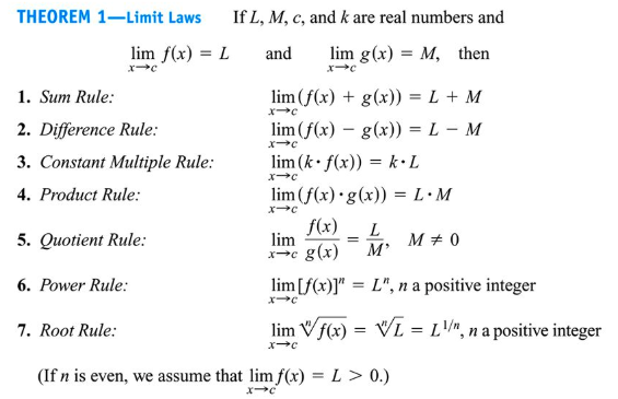
• Use algebraic properties (limit laws) to simplify.
• Use algebraic manipulation (factoring, canceling, rationalizing) to remove removable discontinuities.

The following image (from the original notes) summarizes common algebraic properties:

Limits from graphs: reading behavior

Graph-based limits are about where the graph is headed near $x=a$.

• If both sides head to the same $y$-value, that is the limit.
• If the left and right head to different $y$-values, the two-sided limit does not exist.
• If the graph shoots upward or downward without bound, you have an infinite limit (addressed later).

Worked example: limit exists even when the function value is different

Consider a function with a hole at %%LATEX37%% but the graph approaches %%LATEX38%% from both sides. Then

$\lim_{x\to 2} f(x)=5$

Even if $f(2)$ is undefined (or equals some other value), the limit statement is still about nearby behavior.

Limits from tables: the “trend” skill

Tables test whether you can infer a trend without being fooled by rounding. If values of %%LATEX41%% near %%LATEX42%% look like they approach a stable number, that suggests a finite limit. You should check from both sides when possible.

A common pitfall is over-trusting the table’s value at %%LATEX43%% (if it’s even included). Limits ignore whether %%LATEX44%% actually equals $a$.

Exam Focus

Typical question patterns:

• Estimate limits from a graph or table, including one-sided limits.
• Decide whether a two-sided limit exists by comparing left and right behavior.

Common mistakes:

• Confusing %%LATEX46%% with %%LATEX47%%.
• Declaring “limit does not exist” just because there is a hole or because $f(a)$ is missing.

Limit Laws and Basic Algebraic Evaluation

Once you understand limits conceptually, you need reliable tools to compute them. Limit laws formalize the idea that limits usually behave nicely with arithmetic.

When direct substitution works

To find the limit of a simple polynomial, plug in the number that %%LATEX49%% is approaching. More generally, if %%LATEX50%% is a polynomial, a rational function (with nonzero denominator at the point), an exponential, or many other common functions, you can often find

$\lim_{x\to a} f(x)$

by substituting $x=a$.

Example:

$\lim_{x\to 2} (3x^2-1)=3\cdot 2^2-1=11$

This works because polynomials are continuous everywhere (the continuity idea is developed later, but you can use the fact here).

The key limit laws you actually use

If the limits exist and $c$ is a constant:

$\lim_{x\to a} c=c$

$\lim_{x\to a} \left(f(x)+g(x)\right)=\lim_{x\to a} f(x)+\lim_{x\to a} g(x)$

$\lim_{x\to a} \left(f(x)g(x)\right)=\left(\lim_{x\to a} f(x)\right)\left(\lim_{x\to a} g(x)\right)$

$\lim_{x\to a} \frac{f(x)}{g(x)}=\frac{\lim_{x\to a} f(x)}{\lim_{x\to a} g(x)} \text{ provided } \lim_{x\to a} g(x)\ne 0$

Also useful:

$\lim_{x\to a} \left(f(x)\right)^n=\left(\lim_{x\to a} f(x)\right)^n \text{ for integer } n$

A lot of errors happen when students apply these laws even though a needed limit doesn’t exist, or they ignore the denominator condition in the quotient law.

Indeterminate forms and why they matter

When direct substitution yields

$\frac{0}{0}$

that does not mean the limit is 0 or undefined automatically. It means “the limit requires more work,” because many different behaviors can produce $0/0$.

For example:

• %%LATEX62%% near %%LATEX63%% approaches 1 (even though plugging in gives $0/0$).
• %%LATEX65%% near %%LATEX66%% approaches 0.

Algebraic manipulation: factoring and canceling removable discontinuities

If you get a limit where the denominator becomes 0, factoring is often the first move. You can factor the numerator and denominator, then cancel any removable discontinuities.

For example, in an expression like

$\frac{(x+3)(x+2)}{(x+3)(x-3)}$

the factor %%LATEX68%% can be removed (canceled) for %%LATEX69%%, which corresponds to a removable discontinuity (a hole) at $x=-3$.

A crucial precision point: you are not “canceling terms,” you are canceling common factors, and only after factoring.

Worked example: rational expression with factoring

Evaluate

$\lim_{x\to 3} \frac{x^2-9}{x-3}$

Direct substitution gives $0/0$, so factor:

$x^2-9=(x-3)(x+3)$

Cancel the common factor (valid for $x\ne 3$):

$\frac{(x-3)(x+3)}{x-3}=x+3$

Now substitute:

$\lim_{x\to 3} (x+3)=6$

Conceptually: the original function has a hole at $x=3$, but the values near 3 follow the simplified expression.

Worked example: rationalizing a radical

Evaluate

$\lim_{x\to 0} \frac{\sqrt{x+9}-3}{x}$

Direct substitution gives $0/0$. Multiply by the conjugate:

$\frac{\sqrt{x+9}-3}{x}\cdot \frac{\sqrt{x+9}+3}{\sqrt{x+9}+3}$

Simplify the numerator using difference of squares:

$\frac{(x+9)-9}{x(\sqrt{x+9}+3)}=\frac{x}{x(\sqrt{x+9}+3)}$

Cancel %%LATEX82%% (for %%LATEX83%%) and substitute:

$\lim_{x\to 0} \frac{1}{\sqrt{x+9}+3}=\frac{1}{3+3}=\frac{1}{6}$

A common mistake here is forgetting the conjugate step or incorrectly simplifying the product of conjugates.

Exam Focus

Typical question patterns:

• Evaluate limits that give $0/0$ by factoring, canceling, or rationalizing.
• Use limit laws to break a complicated expression into simpler pieces.

Common mistakes:

• Canceling terms incorrectly (you may cancel common factors, not terms separated by addition).
• Concluding “DNE” immediately from $0/0$ instead of simplifying.

Limit Strategies You Must Recognize (Piecewise, Squeeze Theorem, and Special Trig Limits)

Many AP-style limits aren’t just algebra drills; they test whether you can choose the right strategy. Two very common situations are piecewise definitions and trigonometric expressions.

Limits of piecewise-defined functions

A piecewise function can behave differently depending on whether %%LATEX87%%, %%LATEX88%%, or $x>a$. Limits force you to check approaches from both sides.

If %%LATEX90%% uses “expression 1” for %%LATEX91%% and “expression 2” for $x>a$, then

$\lim_{x\to a^-} f(x)$

uses expression 1, while

$\lim_{x\to a^+} f(x)$

uses expression 2.

Worked example: piecewise limit

Let %%LATEX95%% for %%LATEX96%%, and let %%LATEX97%% for %%LATEX98%%. Find $\lim_{x\to 2} f(x)$.

Left-hand limit:

$\lim_{x\to 2^-} f(x)=\lim_{x\to 2^-} (x+1)=3$

Right-hand limit:

$\lim_{x\to 2^+} f(x)=\lim_{x\to 2^+} (x^2)=4$

Since $3\ne 4$, the two-sided limit does not exist:

$\lim_{x\to 2} f(x) \text{ DNE}$

A frequent misconception is to use the “equals” branch (here, $x^2$) for both sides. Limits care about approach direction, not which formula contains the endpoint.

The Squeeze Theorem (idea and when it applies)

The Squeeze Theorem is for situations where a function is hard to analyze directly, but you can trap it between two easier functions that have the same limit.

Conditions: for all values of %%LATEX105%% in an interval containing %%LATEX106%%,

$g(x)\le f(x)\le h(x)$

and

$\lim_{x\to a} g(x)=L$

$\lim_{x\to a} h(x)=L$

Therefore,

$\lim_{x\to a} f(x)=L$

The intuition is that if the top and bottom boundaries both close in on the same value, the trapped function has nowhere else to go.

Worked example: classic squeeze pattern

Evaluate

$\lim_{x\to 0} x^2 \sin\left(\frac{1}{x}\right)$

For all inputs,

$-1 \le \sin\left(\frac{1}{x}\right) \le 1$

Multiply through by $x^2$ (which is nonnegative):

$-x^2 \le x^2\sin\left(\frac{1}{x}\right) \le x^2$

Now take limits as $x\to 0$:

$\lim_{x\to 0} (-x^2)=0$

$\lim_{x\to 0} x^2=0$

So

$\lim_{x\to 0} x^2 \sin\left(\frac{1}{x}\right)=0$

Special trigonometric limits you should know

A foundational limit is

$\lim_{x\to 0} \frac{\sin x}{x}=1$

A closely related result is

$\lim_{x\to 0} \frac{\tan x}{x}=1$

Other standard trig limits (commonly used by rewriting to match $\sin u/u$) include:

$\lim_{x\to 0} \frac{\cos x-1}{x}=0$

$\lim_{x\to 0} \frac{\sin(ax)}{x}=a$

$\lim_{x\to 0} \frac{\sin(ax)}{\sin(bx)}=\frac{a}{b}$

These aren’t separate “random facts”; they’re patterns you can often derive or justify by algebra plus the base limit $\sin x/x$.

Worked example: using the special trig limit

Evaluate

$\lim_{x\to 0} \frac{\sin(5x)}{x}$

Rewrite to create the exact $\sin u/u$ pattern:

$\frac{\sin(5x)}{x}=5\cdot \frac{\sin(5x)}{5x}$

Then, since %%LATEX129%% as %%LATEX130%%,

$\lim_{x\to 0} 5\cdot \frac{\sin(5x)}{5x}=5\cdot 1=5$

A common mistake is trying to substitute directly and stopping at $0/0$, or forgetting that the denominator must match the sine’s argument.

Exam Focus

Typical question patterns:

• Compute one-sided and two-sided limits for piecewise functions.
• Use the Squeeze Theorem in an oscillating-function setting.
• Evaluate trig limits by rewriting into one of the standard forms above.

Common mistakes:

• Checking only one side for a piecewise limit.
• Misapplying the Squeeze Theorem without showing a valid inequality trap.
• Treating $0/0$ in trig limits as “DNE” instead of rewriting.

Infinite Limits and Asymptotes (Vertical and Horizontal)

Not all limits approach a finite number. Sometimes a function grows without bound as you approach a point (vertical asymptotes), or it has long-run “end behavior” as $x$ becomes very large (horizontal asymptotes).

What an infinite limit means

If

$\lim_{x\to a} f(x)=\infty$

that means as %%LATEX136%% gets close to %%LATEX137%%, $f(x)$ increases without bound. Similarly,

$\lim_{x\to a} f(x)=-\infty$

means it decreases without bound.

This is more informative than vaguely saying “the limit does not exist,” because it tells you exactly how it fails to exist.

Vertical asymptotes via limits

A line %%LATEX140%% is a vertical asymptote of %%LATEX141%% if at least one of these is true:

$\lim_{x\to a^-} f(x)=\infty$

$\lim_{x\to a^-} f(x)=-\infty$

$\lim_{x\to a^+} f(x)=\infty$

$\lim_{x\to a^+} f(x)=-\infty$

You’ll sometimes hear “a vertical asymptote is a line the function cannot cross because the function is undefined there.” The more accurate calculus-level statement is that the function’s values blow up near that line. The function might even be defined at $x=a$ as a single filled point, but the nearby behavior still creates the asymptote.

Worked example: identifying an infinite limit

Evaluate

$\lim_{x\to 2^-} \frac{1}{x-2}$

and

$\lim_{x\to 2^+} \frac{1}{x-2}$

As %%LATEX149%%, %%LATEX150%% is a small negative number, so

$\lim_{x\to 2^-} \frac{1}{x-2}=-\infty$

As %%LATEX152%%, %%LATEX153%% is a small positive number, so

$\lim_{x\to 2^+} \frac{1}{x-2}=\infty$

So $x=2$ is a vertical asymptote, and the two-sided limit does not exist because the sides diverge in opposite directions.

Limits at infinity and horizontal asymptotes

Limits can also describe what happens as $x$ becomes very large:

$\lim_{x\to \infty} f(x)$

$\lim_{x\to -\infty} f(x)$

A line $y=L$ is a horizontal asymptote if:

$\lim_{x\to \infty} f(x)=L$

or

$\lim_{x\to -\infty} f(x)=L$

A key misconception is thinking a function cannot cross a horizontal asymptote. It can; the asymptote is about end behavior far away.

Horizontal asymptote rules for rational functions

For rational functions (ratios of polynomials), end behavior is driven by the highest power of $x$.

• If the highest power of %%LATEX163%% is in the numerator (degree numerator greater than degree denominator), then the limit as %%LATEX164%% approaches infinity is infinity (or negative infinity depending on signs), so there is no horizontal asymptote.
• If the highest power of %%LATEX165%% is in the denominator (degree denominator greater than degree numerator), then the limit as %%LATEX166%% approaches infinity is 0, and the horizontal asymptote is $y=0$.
• If the highest power is the same in numerator and denominator (equal degrees), then the limit is the leading coefficient of the numerator divided by the leading coefficient of the denominator.

Worked example: rational function end behavior

Find

$\lim_{x\to \infty} \frac{3x^2+1}{x^2-5}$

Divide numerator and denominator by $x^2$:

$\frac{3+\frac{1}{x^2}}{1-\frac{5}{x^2}}$

As $x\to \infty$, the fractions go to 0, so

$\lim_{x\to \infty} \frac{3x^2+1}{x^2-5}=\frac{3+0}{1-0}=3$

So %%LATEX173%% is a horizontal asymptote as %%LATEX174%%.

Exam Focus

Typical question patterns:

• Determine infinite limits and identify vertical asymptotes from a graph or algebra.
• Compute limits as $x\to \infty$ for rational functions using dominant terms or degree rules.

Common mistakes:

• Saying “DNE” without specifying %%LATEX176%% or %%LATEX177%% when the function clearly blows up.
• Confusing vertical asymptotes (behavior near a finite %%LATEX178%%-value) with horizontal asymptotes (behavior as %%LATEX179%% grows).
• Assuming asymptotes can never be crossed (horizontal asymptotes can be crossed; vertical asymptotes describe blow-up behavior near a line).

Continuity: Definition, Meaning, and Types of Discontinuities

Limits become especially powerful when connected to continuity, which formalizes when a function has “no breaks” at a point.

What it means for a function to be continuous at a point

A function %%LATEX180%% is continuous at %%LATEX181%% if all three of these are true:

1. $f(a)$ exists.
2. $\lim_{x\to a} f(x)$ exists.
3. $\lim_{x\to a} f(x)=f(a)$.

An intuitive picture is that you can trace the graph near $x=a$ without lifting your pencil, and the “approach value” matches the actual function value.

Continuity on an interval

A function is continuous on an interval if it is continuous at every point on that interval.

• Continuous on %%LATEX186%% means continuous at every point strictly between %%LATEX187%% and $b$.
• Continuous on %%LATEX189%% means continuous on %%LATEX190%% and also continuous from the right at %%LATEX191%% and from the left at %%LATEX192%%.

For endpoints, the limits are one-sided:

$\text{Right-continuous at }a: \lim_{x\to a^+} f(x)=f(a)$

$\text{Left-continuous at }b: \lim_{x\to b^-} f(x)=f(b)$

Types of discontinuities

When continuity fails, naming the type helps you describe what went wrong.

Removable discontinuity (a hole)

An otherwise continuous curve has a hole in it. It’s “removable” because one can remove the discontinuity by filling the hole.

Formally, the limit exists but the function value is missing or doesn’t match the limit:

• $\lim_{x\to a} f(x)=L$ exists
• but either %%LATEX196%% does not exist, or %%LATEX197%%.

Jump discontinuity

Occurs when the curve “breaks” at a particular place and starts somewhere else. The limits from the left and the right both exist, but they do not match:

$\lim_{x\to a^-} f(x) \ne \lim_{x\to a^+} f(x)$

Essential or infinite discontinuity

The curve has a vertical asymptote. At least one one-sided limit is infinite.

Continuity of common function types

You can rely on these facts in typical AP problems:

• Polynomials are continuous for all real inputs.
• Rational functions are continuous wherever the denominator is not zero.
• Many standard functions (exponential, logarithmic, trigonometric) are continuous on their domains.

Continuity under operations

If %%LATEX199%% and %%LATEX200%% are continuous at %%LATEX201%%, then these are also continuous at %%LATEX202%% (where defined): sums, differences, products; quotients when %%LATEX203%%; and compositions (if %%LATEX204%% is continuous at %%LATEX205%% and %%LATEX206%% is continuous at $g(a)$).

This is a major reason direct substitution works so often: continuity lets you replace “approach” with “plug in.”

Removing discontinuities (redefining the function)

You can remove a discontinuity by redefining the function at the troublesome point (effectively changing what happens at that single input). This is frequently done by factoring out a common root between the numerator and denominator, canceling it, and then defining the function’s value at that input to match the limit.

Worked example: choosing a parameter to make a function continuous

Define %%LATEX208%% for %%LATEX209%%, and define $f(1)=k$.

To be continuous at $x=1$, you need

$k=f(1)=\lim_{x\to 1} \frac{x^2-1}{x-1}$

Factor:

$x^2-1=(x-1)(x+1)$

So for $x\ne 1$,

$\frac{x^2-1}{x-1}=x+1$

Then

$\lim_{x\to 1} \frac{x^2-1}{x-1}=\lim_{x\to 1} (x+1)=2$

So

$k=2$

A common mistake is setting %%LATEX218%% equal to the original expression evaluated at %%LATEX219%% (which is undefined). You must simplify first and use the limit.

Exam Focus

Typical question patterns:

• Use the three-part definition to test continuity at a point.
• Determine values of parameters (like $k$) that make a piecewise function continuous.
• Classify discontinuities from a graph or formula.

Common mistakes:

• Assuming a function is discontinuous just because it is piecewise (many piecewise functions are continuous).
• Forgetting that continuity requires both the limit to exist and equality with $f(a)$.

The Intermediate Value Theorem (IVT) and Why Continuity Matters

The Intermediate Value Theorem is a major early payoff of continuity: it lets you guarantee that a function hits certain values without solving the equation exactly.

Intermediate Value Theorem (statement and meaning)

If %%LATEX222%% is continuous on %%LATEX223%% and %%LATEX224%% is any number between %%LATEX225%% and %%LATEX226%%, then there exists at least one %%LATEX227%% in $\left[a,b\right]$ such that

$f(c)=N$

This turns continuity into a guarantee of existence. A helpful mental model is that a continuous function draws a connected curve from %%LATEX230%% to %%LATEX231%%; to get from one height to another without lifting the pencil, it must pass through every height in between.

IVT for showing a root exists

A common use is proving there is a solution to %%LATEX232%% on an interval. If %%LATEX233%% is continuous on %%LATEX234%% and %%LATEX235%% and %%LATEX236%% have opposite signs, then %%LATEX237%% lies between them, so IVT guarantees a point %%LATEX238%% where %%LATEX239%%.

Worked example: guaranteeing a solution

Show that

$x^3+x-1=0$

has a solution in $\left[0,1\right]$.

Let %%LATEX242%%. This is a polynomial, so it is continuous on %%LATEX243%%.

Compute endpoints:

$f(0)=0^3+0-1=-1$

$f(1)=1^3+1-1=1$

Since 0 is between %%LATEX246%% and 1, IVT guarantees there exists %%LATEX247%% in $\left(0,1\right)$ such that

$f(c)=0$

What IVT does not do: it does not tell you the exact value of $c$, and it does not guarantee uniqueness.

IVT and real-world interpretation

If a continuous model represents temperature over time, and it is 60°F in the morning and 80°F in the afternoon, then at some time it must have been 70°F. The continuity requirement is essential; if the function has a jump, it can skip values.

Exam Focus

Typical question patterns:

• Verify IVT hypotheses (continuity on $\left[a,b\right]$) and conclude a solution exists.
• Use sign changes to guarantee a root on an interval.

Common mistakes:

• Forgetting to state continuity (or incorrectly claiming continuity when the function is not defined on the full interval).
• Claiming IVT gives the number of solutions or the exact solution.

Putting It Together: A Deeper Look at “Limit Exists” Questions

Many Unit 1 questions mix skills: reading graphs, checking one-sided behavior, and distinguishing limits from function values. This section ties those threads together in the way AP questions commonly do.

A quick notation reference (limits, values, continuity)

“Does the limit exist?”: the decision process

A two-sided limit exists if you can approach $a$ from both sides and the outputs settle toward the same single number.

Common reasons the two-sided limit does not exist:

1. Jump: left and right approach different finite values.
2. Infinite behavior: one side goes to %%LATEX265%% or %%LATEX266%% (or the sides go to different infinities).
3. Oscillation: values keep fluctuating near $a$ without approaching one number (often seen in functions built from oscillating trig).

Worked example: limit exists but function is not continuous

Suppose %%LATEX268%% for %%LATEX269%%, and $f(1)=10$.

Then the limit is determined by the behavior near 1:

$\lim_{x\to 1} f(x)=\lim_{x\to 1} (x+2)=3$

But $f(1)=10$, so the function is not continuous at 1 even though the limit exists.

Worked example: confirming continuity at an endpoint

If a function is defined on $\left[0,\infty\right)$, you cannot ask for a left-hand limit at 0 in the usual sense because there is no domain to the left. Continuity at 0 is checked with a right-hand limit:

$\lim_{x\to 0^+} f(x)=f(0)$

This idea appears when graphs or piecewise definitions start at an endpoint.

Exam Focus

Typical question patterns:

• Given a graph, report %%LATEX275%%, %%LATEX276%%, %%LATEX277%%, and %%LATEX278%%.
• Decide continuity at a point or on an interval, including endpoint continuity.

Common mistakes:

• Treating any discontinuity as “limit DNE” (removable discontinuities often still have a limit).
• Using a two-sided limit when only a one-sided limit is appropriate (especially at endpoints).
• Mixing up “the limit” with “the function value,” especially when a table includes $x=a$.