Data Analysis & Chance: ACT Statistics Comprehensive Review
Descriptive Statistics: Measures of Center and Spread
Statistics on the ACT Math section often begins with summarizing a set of data using specific values. You need to know not only how to calculate these but how changes to the data affect them.
Measures of Center
These values describe the "middle" or typical value of a dataset.
- Arithmetic Mean (Average): The sum of data values divided by the count of values.
- Median: The middle number when data is ordered from least to greatest. If there is an even number of values, average the two middle numbers.
- Mode: The value that appears most frequently. A set can have no mode, one mode, or multiple modes.
Weighted Average:
The ACT frequently tests weighted averages (e.g., GPA or course grades). You multiply each value by its weight (frequency or percentage), sum them, and divide by the total weight.
Measures of Spread
These describe how spread out or "varied" the data is.
- Range: The simplest measure of spread.
- Standard Deviation: A measure of how much values deviate from the mean. You rarely need to calculate this by hand on the ACT, but you must understand the concept: Higher Standard Deviation = More Spread Out.
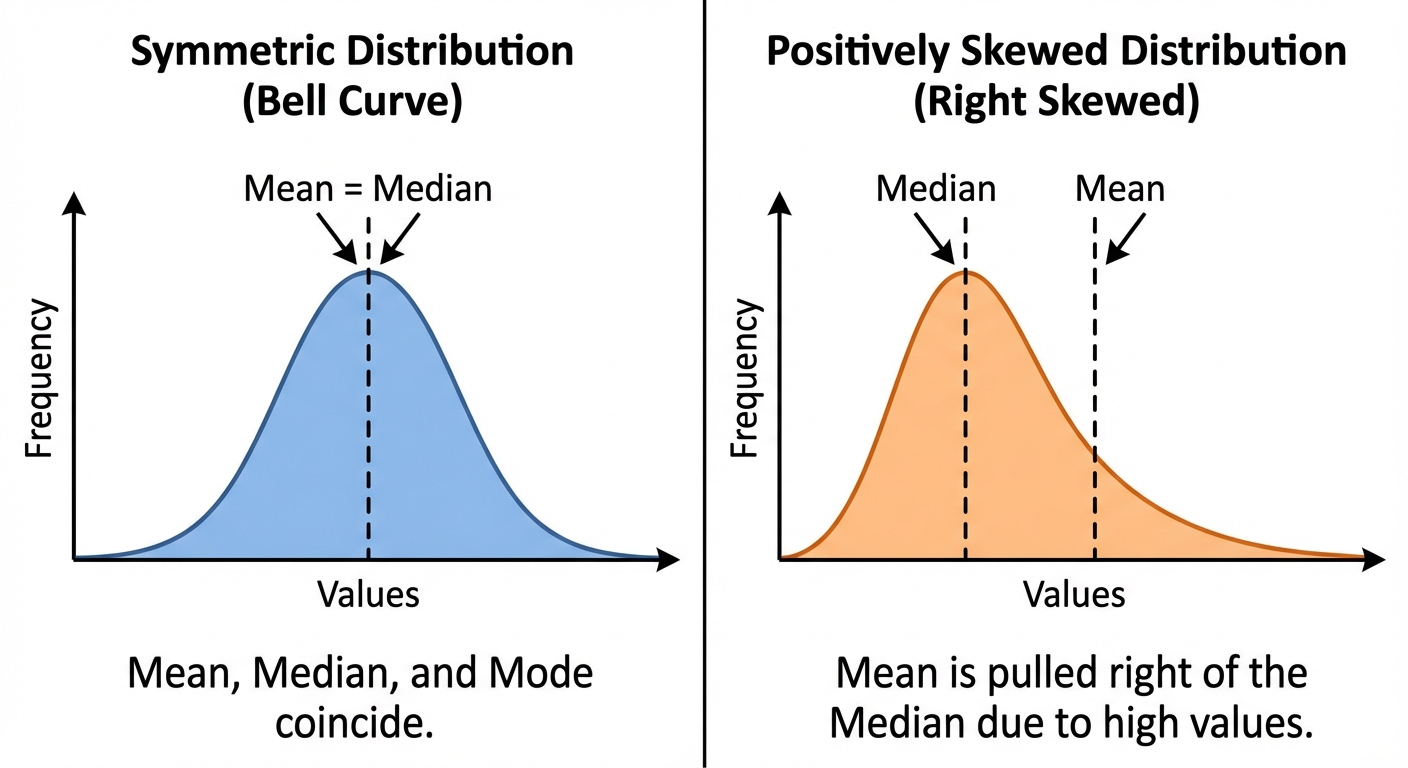
The Impact of Outliers
An outlier is a data point significantly higher or lower than the rest of the data.
- The Mean is sensitive: A high outlier pulls the mean up; a low outlier pulls the mean down.
- The Median is resistant: Outliers generally do not affect the median significantly.
Data Collection Methods and Bias
Occasionally, the ACT asks conceptual questions about how data was gathered. The key to valid statistics is Randomness.
Populations vs. Samples
- Population: The entire group you want to know about (e.g., all high school students in the US).
- Sample: The subset of the group you actually survey (e.g., 500 high school students).
Bias in Surveys
To estimate a population parameter accurately, the sample must be representative.
- Random Sampling: Every member of the population has an equal chance of being selected. This is the gold standard.
- Bias: A systematic error that favors certain outcomes.
- Example: Surveying students in the library about how much they study will likely yield a biased (higher) result compared to the general student body.
Bivariate Data and Scatterplots
Bivariate data involves two variables (usually $x$ and $y$). We use scatterplots to visualize the relationship between them.
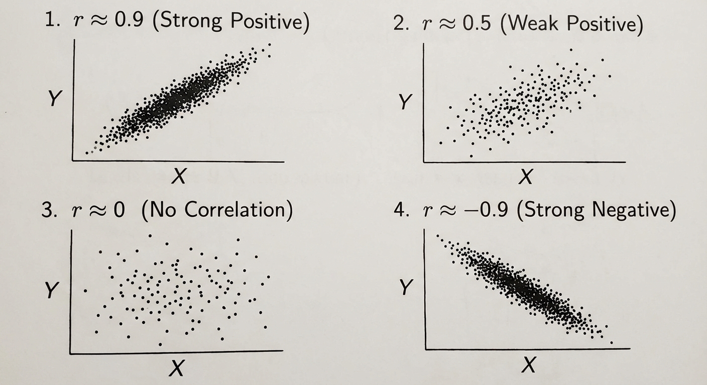
Types of Correlation
Correlation describes the strength and direction of a linear relationship between two quantitative variables.
- Positive Correlation: As $x$ increases, $y$ increases (slope is positive).
- Negative Correlation: As $x$ increases, $y$ decreases (slope is negative).
- No Correlation: Points are scattered randomly with no pattern.
The Correlation Coefficient ($r$)
The value $r$ measures strength and direction. It ranges from $-1$ to $1$.
| Value of $r$ | Interpretation |
|---|---|
| $r \approx 1$ | Strong Positive |
| $r \approx 0.5$ | Weak/Moderate Positive |
| $r \approx 0$ | No Correlation |
| $r \approx -0.5$ | Weak/Moderate Negative |
| $r \approx -1$ | Strong Negative |
Linear and Quadratic Regression
Regression involves fitting a model (equation) to data to make predictions.
Linear Regression (Line of Best Fit)
The line of best fit minimizes the distance between the data points and the line. It is written as:
- Slope ($m$): The predicted change in $y$ for every 1 unit increase in $x$.
- Y-intercept ($b$): The predicted value of $y$ when $x=0$.
Prediction Example:
If a model for plant growth is $h = 2.5d + 4$ (where $h$ is height in cm and $d$ is days), how tall will the plant be in 10 days?
Solution: Substitute $d=10$. $h = 2.5(10) + 4 = 29$ cm.
Quadratic Transformation
Sometimes data looks like a parabola rather than a line. This suggests a quadratic relationship ($y = ax^2 + bx + c$).
- If the data rises then falls, $a$ is negative.
- If the data falls then rises, $a$ is positive.
Calculates Probabilities and Sample Spaces
Probability measures the likelihood of an event occurring, ranging from 0 (impossible) to 1 (certain).
Basic Probability Formula
Counting Principles
To find the "Total Number of Possible Outcomes" (the Sample Space), use the Fundamental Counting Principle.
- Rule: If there are $a$ ways to do task A and $b$ ways to do task B, there are $a \times b$ ways to do both.
Example: A diner offers 3 appetizers, 5 entrees, and 2 desserts. How many different 3-course meals can be ordered?
Compound Events
- Independent Events (AND): If the outcome of one event does not affect the other.
- Mutually Exclusive Events (OR): Events that cannot happen at the same time.
- General Addition Rule (Overlapping Events): If events can happen at the same time (e.g., pulling a Red card OR a King), you must subtract the overlap.
Geometric Probability
Sometimes probability is visual. If you throw a dart at a board:
Normal Distributions
The ACT occasionally tests the specific properties of the Normal Distribution (Bell Curve). These distributions are symmetric, and the Mean = Median = Mode.
The Empirical Rule (68-95-99.7)
Data in a normal distribution follows a specific pattern based on standard deviations ($\sigma$) from the mean ($\mu$).
- 68% of data falls within 1 standard deviation of the mean.
- 95% of data falls within 2 standard deviations of the mean.
- 99.7% of data falls within 3 standard deviations of the mean.
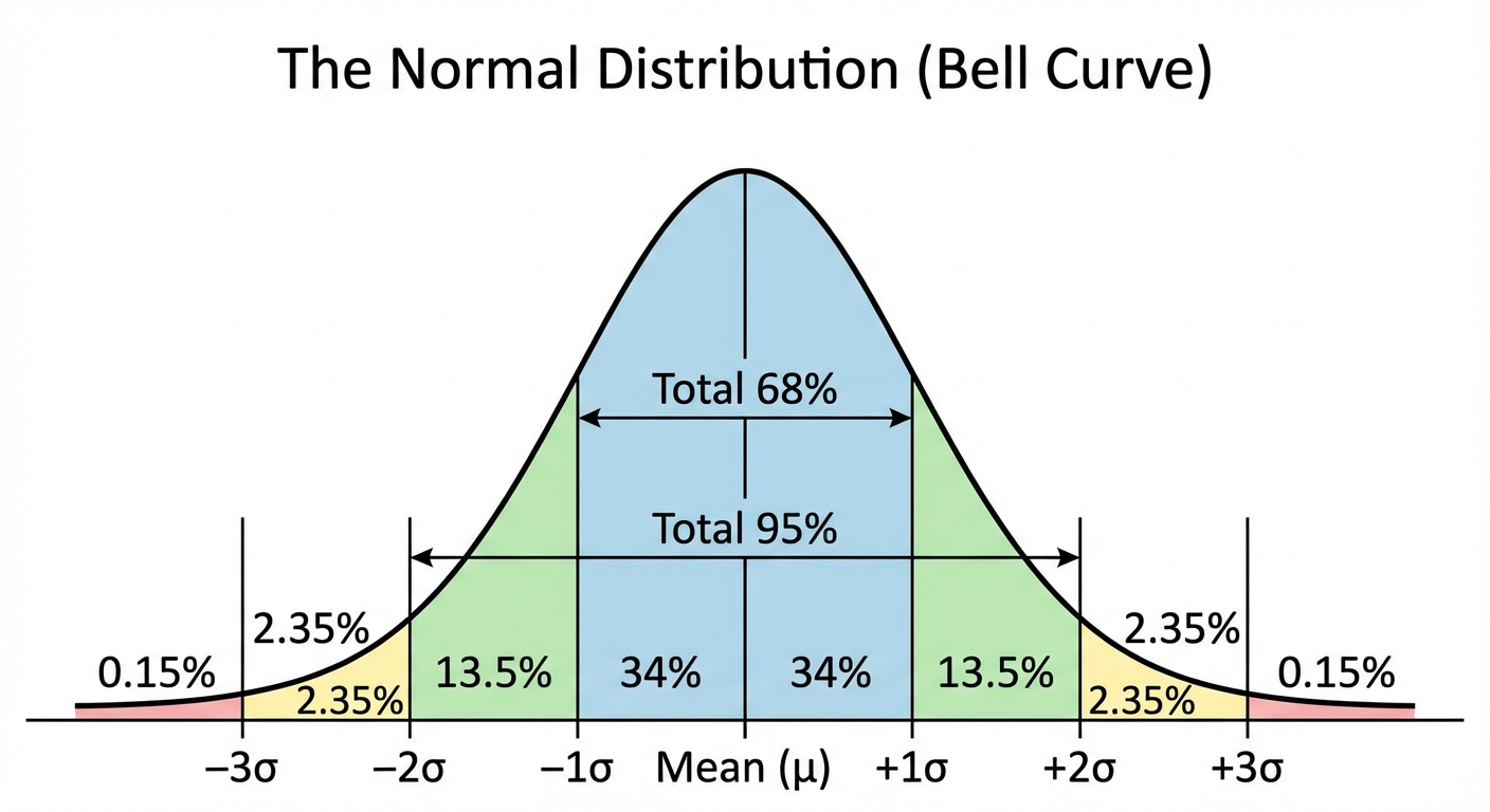
Worked Example:
The scores on a standardized test are normally distributed with a mean of 500 and a standard deviation of 100. What percent of students score between 400 and 600?
- 400 is $500 - 100$ (-1 SD).
- 600 is $500 + 100$ (+1 SD).
- The area between -1 SD and +1 SD is 68%.
Common Mistakes & Pitfalls
Confusing Mean and Median:
- Mistake: Using the average when looking for the "middle" of a skewed dataset.
- Correction: Check for outliers. If the data is heavily skewed, the median is a better representation of the center.
Misinterpreting Correlation vs. Causation:
- Mistake: Assuming that because $x$ and $y$ are strongly correlated, $x$ causes $y$.
- Correction: Correlation simply measures association. A third variable could be influencing both.
Forgetting to Order Data for Median:
- Mistake: Finding the middle number of an unsorted list.
- Correction: Always sort the list from least to greatest first!
Double Counting in Probability:
- Mistake: Adding probabilities for "OR" questions without subtracting the overlap.
- Correction: Use the formula $P(A \cup B) = P(A) + P(B) - P(A \cap B)$. Always check if a card can be both "Red" and a "King".
The "At Least One" Trick:
- Mistake: Trying to calculate $P(\text{1}) + P(\text{2}) + P(\text{3})…$ which is time-consuming.
- Correction: The probability of "at least one" is $1 - P(\text{None})$.