Comprehensive Guide to Trigonometric & Polar Functions
3.1 Periodic Phenomena
Understanding Periodicity
Periodic Phenomena describe events or processes that repeat in identical intervals of time or space. In the real world, this includes tides, planetary orbits, heartbeats, and the vibration of guitar strings.
From a mathematical perspective, a function $f$ is periodic if there is a positive number $p$ such that:
for all $x$ in the domain. The smallest distinct positive value of $p$ is called the period.
Key Features of Periodic Graphs
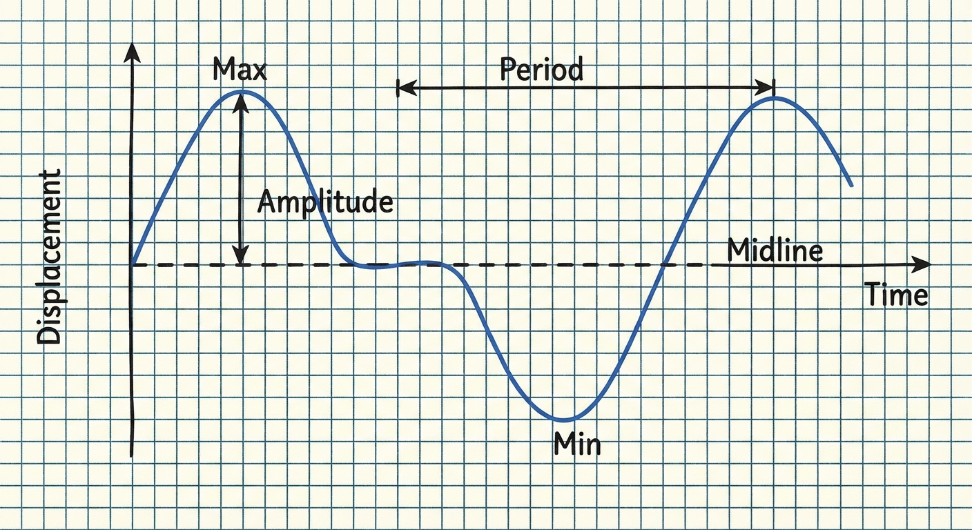
When analyzing the graph of a periodic function (like the height of a Ferris wheel carriage over time), we identify several structural components:
- Cycle: One complete repetition of the pattern.
- Period: The horizontal length (interval) of one complete cycle.
- Midline: The horizontal line that runs exactly in the middle of the graph's maximum and minimum values. It represents the vertical centered position.
- Amplitude: The vertical distance from the midline to a maximum (or minimum). It indicates the "strength" or height of the wave.
- Concavity: Indicates how the rate of change is changing.
- Concave Up: The graph bends upward (like a cup). The rate of change is increasing.
- Concave Down: The graph bends downward (like a frown). The rate of change is decreasing.
3.2 Sine, Cosine, and Tangent (Geometric Definitions)
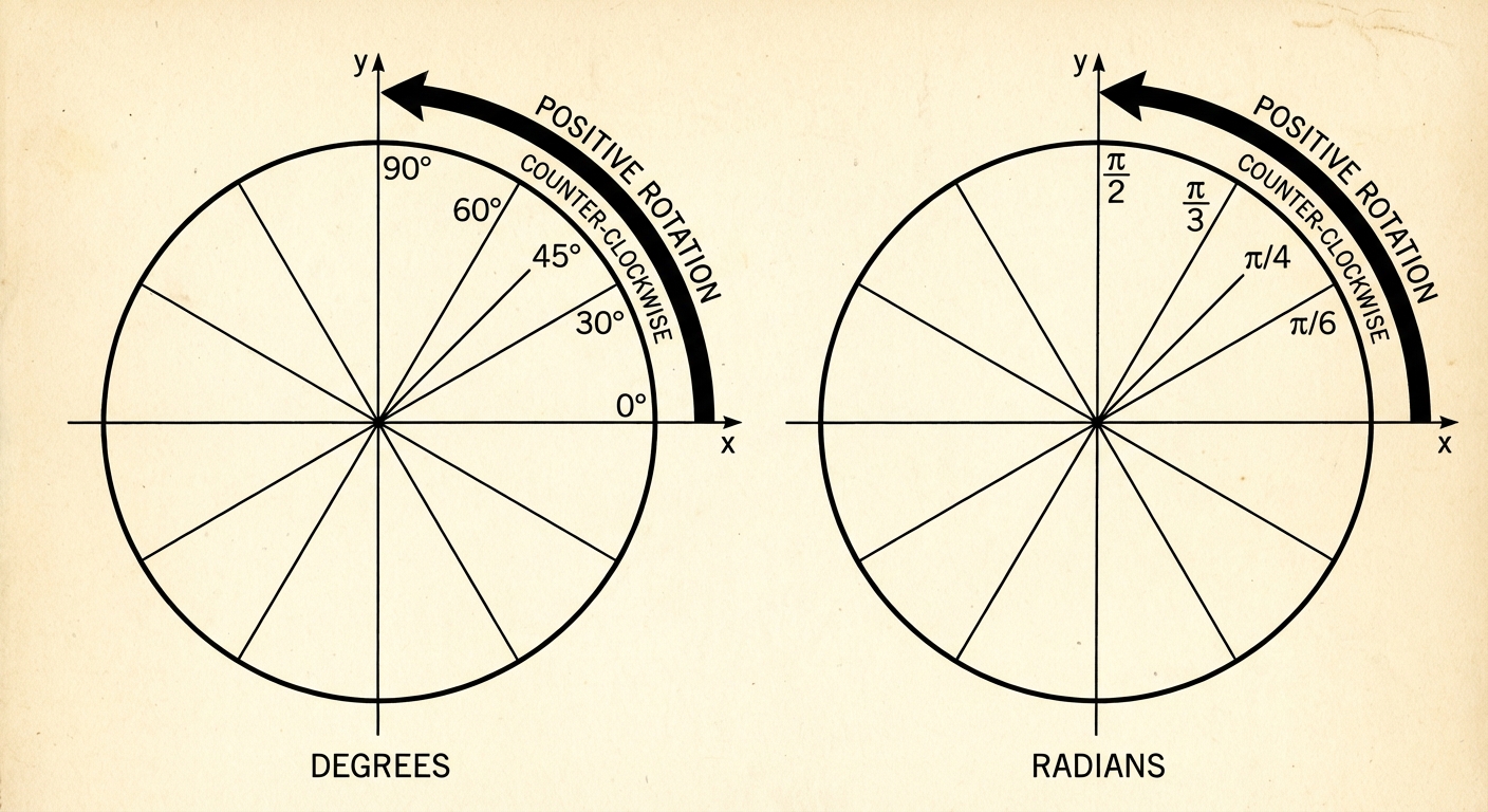
Standard Position
To model periodicity mathematically, we use the coordinate plane. An angle $\theta$ is in Standard Position when:
- Its vertex is at the origin $(0,0)$.
- Its initial side lies along the positive x-axis.
Rotation determines the sign:
- Positive Angle: Counter-clockwise rotation.
- Negative Angle: Clockwise rotation.
Coterminal Angles
Angles that end at the same terminal side but differ by full rotations are coterminal.
- Equation: $\theta_{coterminal} = \theta \pm 360^\circ n$ or $\theta \pm 2\pi n$.
- Example: $30^\circ$ and $390^\circ$ are coterminal.
Radians vs. Degrees
AP Precalculus primarily uses radians because they relate angle measure directly to arc length.
- Definition: One radian is the angle subtended by an arc equal in length to the radius of the circle.
- Formula: $\theta = \frac{s}{r}$, where $s$ is arc length and $r$ is radius.
- Conversion: $\pi \text{ radians} = 180^\circ$.
The Unit Circle Definitions
The Unit Circle is a circle with radius $r=1$ centered at the origin ($x^2 + y^2 = 1$). For any angle $\theta$ in standard position intersecting the unit circle at point $(x, y)$:
- $\cos(\theta) = x$
- $\sin(\theta) = y$
- $\tan(\theta) = \frac{y}{x} = \frac{\sin(\theta)}{\cos(\theta)}$ (Slope of the terminal ray)
3.3 Sine and Cosine Function Values
Major Quadrant Values
Values on the axes ($0, \frac{\pi}{2}, \pi, \frac{3\pi}{2}$) correspond to coordinates $(1,0), (0,1), (-1,0), (0,-1)$.
Special Right Triangles
To determine exact values for non-axial angles, we rely on geometry:
- 30-60-90 Triangle ($\frac{\pi}{6}, \frac{\pi}{3}, \frac{\pi}{2}$)
- Sides: $1 : \sqrt{3} : 2$ (hypotenuse). On Unit Circle ($r=1$), sides are $\frac{1}{2}$ and $\frac{\sqrt{3}}{2}$.
- 45-45-90 Triangle ($\frac{\pi}{4}, \frac{\pi}{4}, \frac{\pi}{2}$)
- Sides: $1 : 1 : \sqrt{2}$. On Unit Circle, sides are $\frac{\sqrt{2}}{2}$.
The Reference Angle Rule
To find values for angles > 90°:
- Find the Reference Angle (acute angle formed by the terminal side and the x-axis).
- Determine the value based on special triangles.
- Determine the sign (+/-) based on the quadrant (ASTC: All Students Take Calculus).
- Q1: All positive.
- Q2: Sine positive.
- Q3: Tangent positive.
- Q4: Cosine positive.
3.4 Sinusoidal Functions (Graphs)
We transition from the unit circle (input: angle, output: coordinates) to functional graphs (input: $x$ or $\theta$, output: $y$).
The Sine Graph ($f(x) = \sin x$)
- Starts at: Midline (0,0) going up.
- Domain: $(-\infty, \infty)$
- Range: $[-1, 1]$
- Symmetry: Odd Function (Symmetric about origin). $\sin(-x) = -\sin(x)$.
The Cosine Graph ($f(x) = \cos x$)
- Starts at: Extremum (0,1) going down.
- Domain: $(-\infty, \infty)$
- Range: $[-1, 1]$
- Symmetry: Even Function (Symmetric about y-axis). $\cos(-x) = \cos(x)$.
Note: Graphs are identical in shape but shifted by $\frac{\pi}{2}$ horizontally.
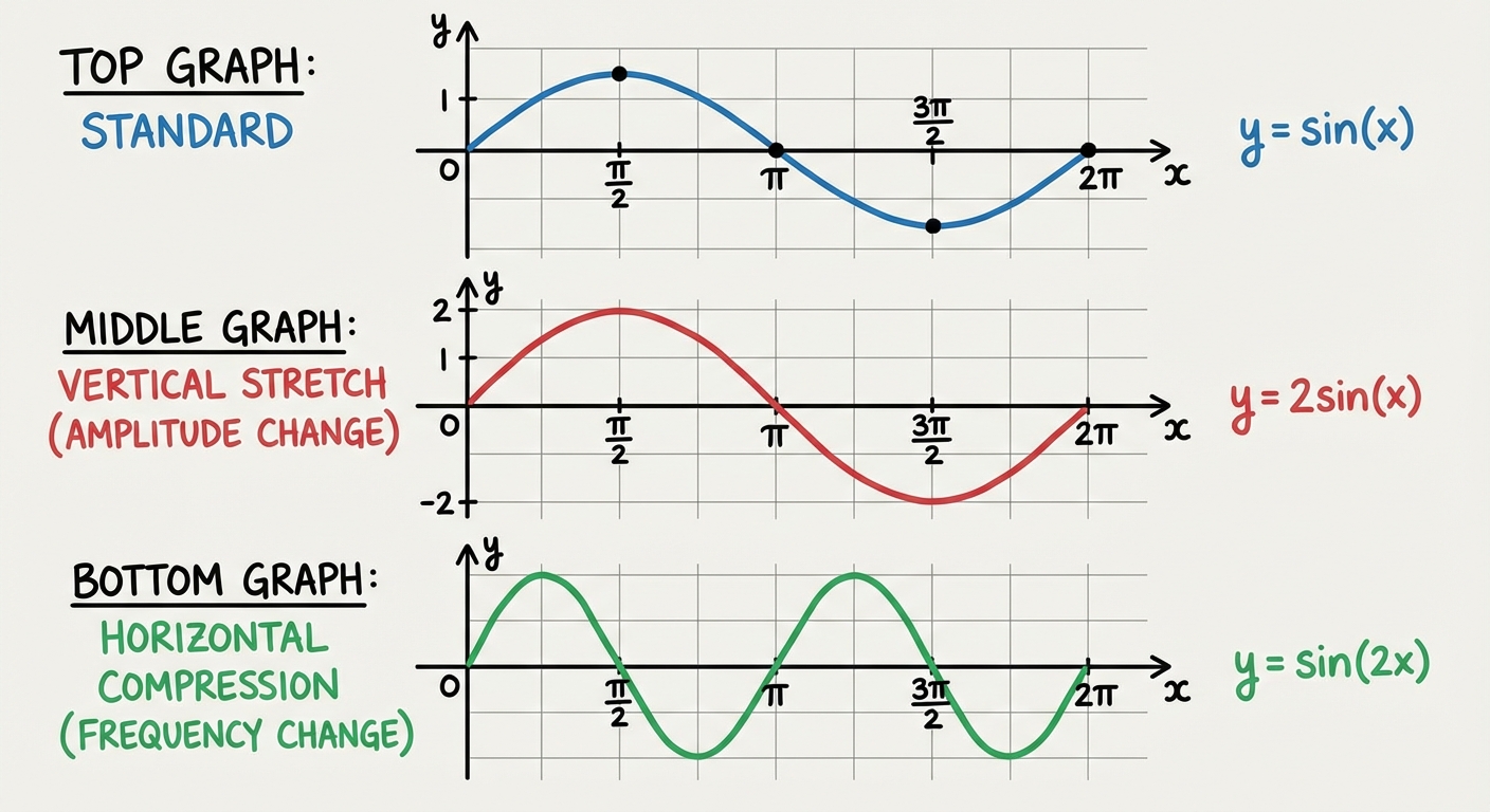
3.5 & 3.6 Sinusoidal Transformations
The general form for sine and cosine functions is:
Transformation Parameters
| Parameter | Mathematical Effect | Graph Feature |
|---|---|---|
| **$ | a | $** |
| $a < 0$ | Reflection over midline | Flips the shape. |
| **$ | b | $** |
| $c$ | Horizontal Shift | Phase Shift. Shifts right if $x-c$, left if $x+c$. |
| $d$ | Vertical Shift | Midline. $y=d$. |
Analyzing Frequency
Frequency is the number of cycles per unit interval of input. In physics contexts (time), frequency is the reciprocal of the period:
Steps to Graph
- Draw the Midline ($y=d$).
- Mark Max/Min lines using Amplitude ($d \pm a$).
- Determine Period ($2\pi/b$) and mark the end of one cycle starting from $c$.
- Divide the period into 4 equal segments (quarter-points).
- Plot key points (intercepts, max, min) based on Sine (mid-max-mid-min-mid) or Cosine (max-mid-min-mid-max) patterns.
3.7 Context and Data Modeling
When given real-world data (e.g., tides, temperature, pendulum swing):
- Find Midline ($d$): Average of maximum and minimum data vales.
- Find Amplitude ($a$): Distance from max to midline.
- Find Period ($P$): Time it takes to go from Max to Max (or Min to Min). If given Max to Min, that is only half the period.
- Find $b$: $b = \frac{2\pi}{P}$.
- Find Phase Shift ($c$):
- For Cosine: The $x$-value of the first Maximum.
- For Sine: The $x$-value where the graph crosses the midline going up.
- Tip: It is usually easier to model data using negative Cosine (starting at min) or positive Cosine (starting at max) than Sine, as peaks are easier to spot than inflection points.
Common Mistakes (Sinusoidals)
- Forgeting to factor out $b$: In $y = \sin(2x - \pi)$, the shift is NOT $\pi$. You must factor: $\sin(2(x - \frac{\pi}{2}))$. The shift is $\frac{\pi}{2}$.
- Degrees vs Radians: Calculus and most AP Precalc graphing questions assume Radians unless units are explicitly "degrees".
3.8 The Tangent Function
The function $f(x) = \tan(x) = \frac{\sin x}{\cos x}$ behaves differently because the denominator can be zero.
Key Features
- Period: $\pi$ (repeats twice as fast as sin/cos).
- Asymptotes: Occur where $\cos x = 0$. Vertical asymptotes at $x = \frac{\pi}{2} + n\pi$.
- Range: $(-\infty, \infty)$. No amplitude.
- X-Intercepts: Where $\sin x = 0$ (at $n\pi$).
Transformations
- Period: $\frac{\pi}{|b|}$ (Note: use $\pi$, not $2\pi$).
- Asymptotes: Found by solving $b(x-c) = \pm \frac{\pi}{2}$.
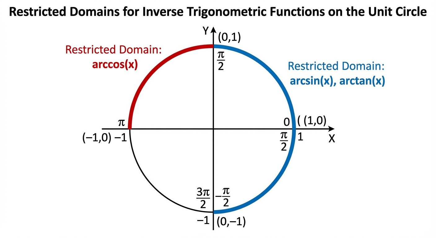
3.9 Inverse Trigonometric Functions
To define an inverse function, the original function must be one-to-one (pass the horizontal line test). Trig functions fail this, so we must restrict their domains.
The Inverse Functions
Inverse Sine ($y = \sin^{-1}x$ or $\arcsin x$)
- Restricted Domain of sin: $[-\frac{\pi}{2}, \frac{\pi}{2}]$ (Quadrant 4 and 1).
- Domain of arcsin: $[-1, 1]$.
- Range of arcsin: $[-\frac{\pi}{2}, \frac{\pi}{2}]$.
- Interpretation: "The angle between $-\pi/2$ and $\pi/2$ whose sine is $x$."
Inverse Cosine ($y = \cos^{-1}x$ or $\arccos x$)
- Restricted Domain of cos: $[0, \pi]$ (Quadrant 1 and 2).
- Domain of arccos: $[-1, 1]$.
- Range of arccos: $[0, \pi]$.
Inverse Tangent ($y = \tan^{-1}x$ or $\arctan x$)
- Restricted Domain of tan: $(-\frac{\pi}{2}, \frac{\pi}{2})$.
- Domain of arctan: $(-\infty, \infty)$.
- Range of arctan: $(-\frac{\pi}{2}, \frac{\pi}{2})$.
3.10 Trigonometric Equations and Inequalities
Solving Strategies
- Isolate the Trig Function: Get $\sin(x) = k$ by itself.
- Find the Reference Angle: Ignore the negative sign of $k$ initially to find the acute angle $\alpha$.
- Place in Quadrants: Use the sign of $k$ to determine valid quadrants.
- General Solutions:
- For Sin/Cos: Add $+ 2\pi n$ to specific solutions.
- For Tan: Add $+ \pi n$ to the specific solution.
Example: Solve $2\sin(x) + 1 = 0$ on $[0, 2\pi)$.
- $\sin(x) = -\frac{1}{2}$.
- Ref angle for $1/2$ is $\frac{\pi}{6}$.
- Sine is negative in Q3 and Q4.
- Q3: $\pi + \frac{\pi}{6} = \frac{7\pi}{6}$. Q4: $2\pi - \frac{\pi}{6} = \frac{11\pi}{6}$.
3.11 Secant, Cosecant, and Cotangent
These are reciprocal functions. Their graphs generally form "U" shapes opening away from the base sine/cosine/tangent graphs, separated by asymptotes.
| Function | Definition | Asymptotes (where denom = 0) |
|---|---|---|
| Cosecant | $\csc \theta = \frac{1}{\sin \theta}$ | $x = n\pi$ |
| Secant | $\sec \theta = \frac{1}{\cos \theta}$ | $x = \frac{\pi}{2} + n\pi$ |
| Cotangent | $\cot \theta = \frac{\cos \theta}{\sin \theta}$ | $x = n\pi$ |
Common Mistake: Confusing which is the reciprocal of which. Remember: Secant goes with Cosine, Cosecant goes with Sine.
3.12 Identities
For AP Precalculus, you must be proficient with the following representations to simplify expressions and solve equations.
1. Pythagorean Identities
Derived from $x^2 + y^2 = 1$ on the unit circle.
- $\sin^2\theta + \cos^2\theta = 1$ (Most important)
- $\tan^2\theta + 1 = \sec^2\theta$
- $1 + \cot^2\theta = \csc^2\theta$
2. Sum and Difference Formula
Useful for finding exact values of angles like $15^\circ$ ($45-30$) or $75^\circ$ ($45+30$).
- $\sin(A \pm B) = \sin A \cos B \pm \cos A \sin B$
- $\cos(A \pm B) = \cos A \cos B \mp \sin A \sin B$ (Note the sign flip!)
3.13 Polar Coordinates
In the Polar system, a point is defined by $(r, \theta)$, where $r$ is the directed distance from the origin (pole) and $\theta$ is the angle of rotation from the positive x-axis (polar axis).
Conversion Formulas
Converting between Polar $(r, \theta)$ and Rectangular $(x, y)$:
Polar $\to$ Rectangular:
- $x = r\cos\theta$
- $y = r\sin\theta$
Rectangular $\to$ Polar:
- $r^2 = x^2 + y^2 \implies r = \pm\sqrt{x^2+y^2}$
- $\tan\theta = \frac{y}{x}$
Note on Non-Uniqueness: Unlike $(x,y)$, polar coordinates are not unique. $(r, \theta)$ is the same point as $(r, \theta + 2\pi)$ and $(-r, \theta + \pi)$.
3.14 Polar Function Graphs
1. Circles
- $r = a$: Centered at origin, radius $a$.
- $r = a\cos\theta$: Diameter $a$, symmetric along x-axis (horizontal).
- $r = a\sin\theta$: Diameter $a$, symmetric along y-axis (vertical).
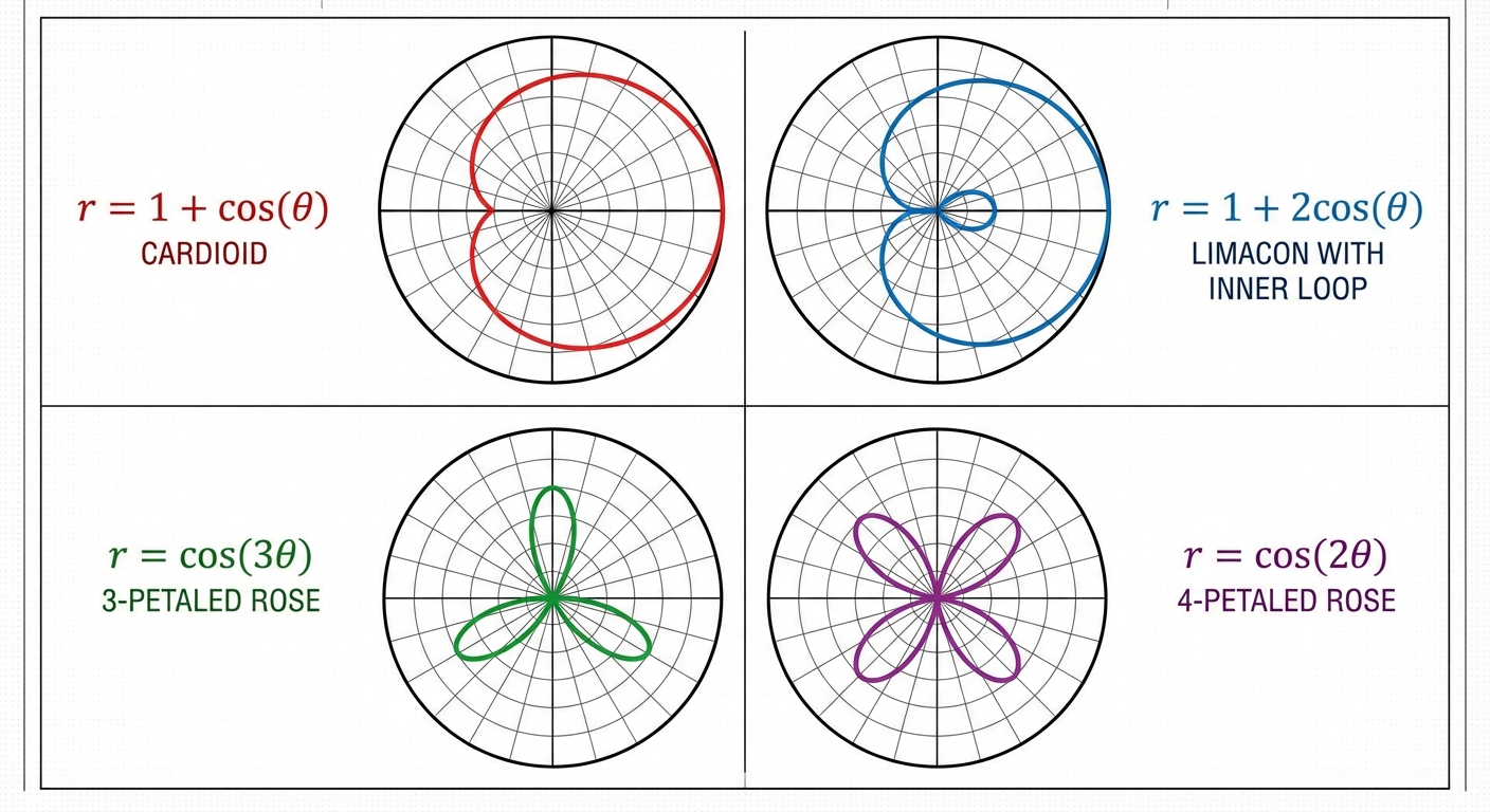
2. Limaçons
General Form: $r = a \pm b\cos\theta$ or $r = a \pm b\sin\theta$. ($a>0, b>0$)
The ratio $\frac{a}{b}$ determines the shape:
- $\frac{a}{b} < 1$ (Loop): The graph passes through the pole and has an inner loop.
- $\frac{a}{b} = 1$ (Cardioid): Heart-shaped. Touches the pole (cusp) but no loop.
- $1 < \frac{a}{b} < 2$ (Dimpled): Has a "dent" but does not touch the pole.
- $\frac{a}{b} \ge 2$ (Convex): Almost round, slightly flattened on one side.
3. Roses
General Form: $r = a\cos(n\theta)$ or $r = a\sin(n\theta)$.
- If $n$ is odd: The rose has $n$ petals.
- If $n$ is even: The rose has $2n$ petals.
3.15 Rates of Change in Polar Functions
We analyze how the distance from the origin, $r$, changes as the angle $\theta$ changes.
Average Rate of Change
Interpreting the Sign
- If $\frac{dr}{d\theta} > 0$ (Increasing): As the angle rotates counter-clockwise, the point moves further from the origin (if $r > 0$).
- If $\frac{dr}{d\theta} < 0$ (Decreasing): As the angle rotates, the point moves closer to the origin (if $r > 0$).
- Extrema: When rate of change transitions from positive to negative, the function reaches a relative maximum distance from the pole. If $r=0$, the graph passes through the pole.
Crucial Concept: This is not dy/dx (slope of the curve). It is the rate at which the radius grows or shrinks.